
如果你也在 怎样代写国际经济学International Economics 这个学科遇到相关的难题,请随时右上角联系我们的24/7代写客服。国际经济学International Economics关注的是生产资源和消费者偏好的国际差异对经济活动的影响,以及影响它们的国际机构。它试图解释不同国家的居民之间的交易和互动的模式和后果,包括贸易、投资和交易。
国际经济学International Economics从供需因素、经济一体化、国际要素流动和政策变量(如关税率和贸易配额)等方面研究商品和服务在国际边界的流动。国际金融研究资本在国际金融市场上的流动,以及这些流动对汇率的影响。国际货币经济学和国际宏观经济学研究货币在各国之间的流动,以及由此对各国经济整体的影响。国际政治经济学是国际关系的一个分支,研究国际冲突、国际谈判和国际制裁等问题和影响;国家安全和经济民族主义;以及国际协议和遵守情况。
国际经济学International Economics代写,免费提交作业要求, 满意后付款,成绩80\%以下全额退款,安全省心无顾虑。专业硕 博写手团队,所有订单可靠准时,保证 100% 原创。最高质量的国际经济学International Economics作业代写,服务覆盖北美、欧洲、澳洲等 国家。 在代写价格方面,考虑到同学们的经济条件,在保障代写质量的前提下,我们为客户提供最合理的价格。 由于作业种类很多,同时其中的大部分作业在字数上都没有具体要求,因此国际经济学International Economics作业代写的价格不固定。通常在专家查看完作业要求之后会给出报价。作业难度和截止日期对价格也有很大的影响。
同学们在留学期间,都对各式各样的作业考试很是头疼,如果你无从下手,不如考虑my-assignmentexpert™!
my-assignmentexpert™提供最专业的一站式服务:Essay代写,Dissertation代写,Assignment代写,Paper代写,Proposal代写,Proposal代写,Literature Review代写,Online Course,Exam代考等等。my-assignmentexpert™专注为留学生提供Essay代写服务,拥有各个专业的博硕教师团队帮您代写,免费修改及辅导,保证成果完成的效率和质量。同时有多家检测平台帐号,包括Turnitin高级账户,检测论文不会留痕,写好后检测修改,放心可靠,经得起任何考验!
想知道您作业确定的价格吗? 免费下单以相关学科的专家能了解具体的要求之后在1-3个小时就提出价格。专家的 报价比上列的价格能便宜好几倍。
经济代写|国际经济学代写International Economics代考|Outline of the Formal Derivation of Nation 2’s Offer Curve
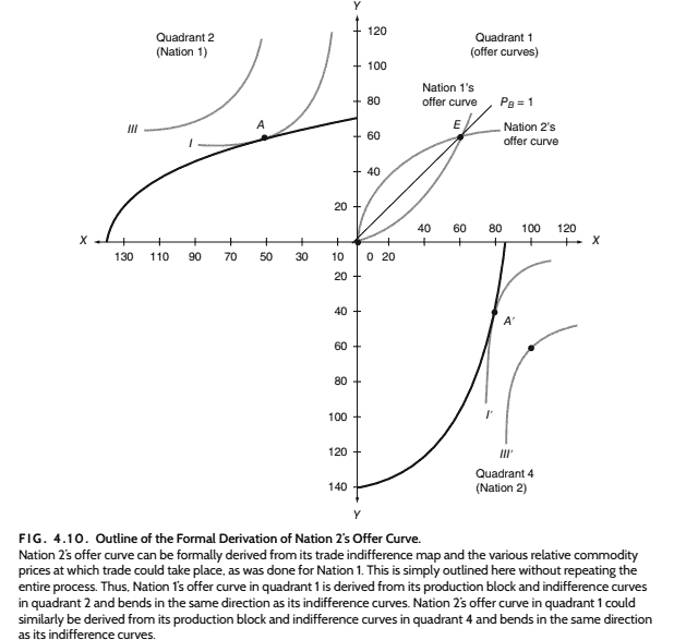
Nation 2’s offer curve can be formally derived in a completely analogous way from its trade indifference map and the various relative commodity prices at which trade could take place. This is outlined in Figure 4.10 without repeating the entire process.
Quadrant 2 of Figure 4.10 shows Nation 1’s production frontier, or block, and indifference curves $I$ and $I I I$, while quadrant 4 shows the same things for Nation 2. Nation 2’s production frontier and indifference curves are placed in quadrant 4 so that its offer curve will be derived in the proper relationship to Nation 1’s offer curve in quadrant 1.
Nation 1’s offer curve in quadrant 1 of Figure 4.10 was derived from its trade indifference map in Figure 4.9. Note that Nation 1’s offer curve bends in the same direction as its community indifference curves. In a completely analogous way, Nation 2’s offer curve in quadrant 1 of Figure 4.10 can be derived from its trade indifference map and bends in the same direction as its community indifference curves in quadrant 4 .
The offer curves of Nation 1 and Nation 2 in quadrant 1 of Figure 4.10 are the offer curves of Figure 4.5 and define the equilibrium-relative commodity price of $P_B=1$ at their intersection. As will be seen in the next section, only at point $E$ does general equilibrium exist.
Problem Draw a figure showing Nation 2’s trade indifference curves that would give its offer curve, including its backward-bending portion.
经济代写|国际经济学代写International Economics代考|General Equilibrium of Production, Consumption, and Trade
Figure 4.11 brings together in one diagram all the information about production, consumption, and trade for the two nations in equilibrium. The production blocks of Nation 1 and Nation 2 are joined at point $E^*$ (the same as point $E$ in Figure 4.10), where the offer curves of the two nations cross.
With trade, Nation 1 produces $130 \mathrm{X}$ and $20 \mathrm{Y}$ (point $E$ with reference to point $E^$ ) and consumes $70 \mathrm{X}$ and $80 \mathrm{Y}$ (the same point $E$ but with reference to the origin, $O$ ) by exchanging $60 \mathrm{X}$ and $60 \mathrm{Y}$ with Nation 2. On the other hand, Nation 2 produces $40 \mathrm{X}$ and $120 \mathrm{Y}$ (point $E^{\prime}$ with reference to point $E^$ ) and consumes $100 \mathrm{X}$ and $60 \mathrm{Y}$ (the same point $E^{\prime}$ but with reference to the origin) by exchanging $60 \mathrm{Y}$ for $60 \mathrm{X}$ with Nation 1 .
International trade is in equilibrium with $60 \mathrm{X}$ exchanged for $60 \mathrm{Y}$ at $P_B=1$. This is shown by the intersection of offer curves 1 and 2 at point $E^* . P_B=1$ is also the relative commodity price of $\mathrm{X}$ prevailing domestically in Nation 1 and Nation 2 (see the relative price line tangent to each nation’s production blocks at points $E$ and $E^{\prime}$, respectively). Thus, producers, consumers, and traders in both nations all respond to the same set of equilibriumrelative commodity prices.
Note that point $E$ on Nation 1’s indifference curve $I I I$ measures consumption in relation to the origin, $O$, while the same point $E$ on Nation 1’s production block measures production from point $E^*$. Finding Nation 1 ‘s indifference curve $I I I$ tangent to its production block at point $E$ seems different but is in fact entirely consistent and confirms the results of Figure 3.4 for Nation 1. The same is true for Nation 2 .
Figure 4.11 summarizes and confirms all of our previous results and the conclusions of our trade model (compare, for example, Figure 4.11 with Figure 3.4). Thus, Figure 4.11 is a complete general equilibrium model (except for the fact that it deals with only two nations and two commodities). The figure is admittedly complicated. But this is because it summarizes in a single graph a tremendous amount of very useful information. Figure 4.11 is the pinnacle of the neoclassical trade model. The rewards of mastering it are great indeed in terms of future deeper understanding.

国际经济学代写
经济代写|国际经济学代写INTERNATIONAL ECONOMICS代考|OUTLINE OF THE FORMAL DERIVATION OF NATION 2’S OFFER CURVE
国家 2 的报价曲线可以通过完全类似的方式从其贸易无差异图和可能发生贸易的各种相对商品价格中正式导出。图 4.10对此进行了概述,但末重 复整个过程。
图 4.10 的象限 2 显示了国家 1 的生产边界或块和无差异曲线 $I$ 和 $I I I$ ,而第 4 象限显示了国家 2 的相同情况。国家 2 的生产边界和无差异曲线位于 第 4 象限,因此其供给曲线将根据与第 1 象限中国家 1 的供给曲线的适当关系导出。
图 4.10 象限 1 中国家 1 的供给曲线来自图 4.9 中的贸易无差异图。请注意,国家 1 的供给曲线与其社区无差异曲线的弯曲方向相同。以完全类似的 方式,国家 2 在图 4.10 的象限 1 中的供给曲线可以从其贸易无差异图导出,并与象限 4 中的社区无差异曲线向同一方向弯曲。
图 4.10 象限 1 中国家 1 和国家 2 的报价曲线是图 4.5 的报价曲线,并定义均衡相对商品价格 $P_B=1$ 在他们的路口。正如将在下一节中看到的那 样,仅在点 $E$ 一般均衡是否存在。
问题画出国家 2 的贸易无差异曲线图,给出其供给曲线,包括向后弯曲的部分。
经济代写|国际经济学代写INTERNATIONAL ECONOMICS代考|GENERAL EQUILIBRIUM OF PRODUCTION, CONSUMPTION, AND TRADE
图 4.11 将两国处于均衡状态的生产、消费和贸易的所有信息汇总在一张图中。Nation 1 和 Nation 2 的生产块在点处连接 $E^$ thesameaspoint $\$$ \$inFigure4.10,两国的报价曲线相交。 通过贸易,Nation 1生产 $130 \mathrm{X}$ 和 $20 \mathrm{Y}$ point $\$ E \$$ withreferencetopoint $\$ E^{\$}$ 并消耗 $70 \mathrm{X}$ 和 $80 \mathrm{Y}$ thesamepoint $\$$ Ebutwithreferencetotheorigin, $\$ O \$$ 通过交换 $60 \mathrm{X}$ 和 $60 \mathrm{Y}$ 与国家 2. 另一方面,国家 2 生产 $40 \mathrm{X}$ 和 $120 \mathrm{Y}$ point $\$ E^{\prime} \$$ withreferencetopoint $\$ E^8$ 并消耗 $100 \mathrm{X}$ 和 $60 \mathrm{Y}$ thesamepoint $\$ E^{\prime} \$$ butwithreferencetotheorigin通过交换 $60 \mathrm{Y}$ 为了60X 与国家 1 o 国际贸易与 $60 \mathrm{X}$ 换来的 $60 \mathrm{Y}$ 在 $P_B=1$. 这由报价曲线 1 和 2 在点处的交点显示 $E^ \cdot P_B=1$ 也是商品的相对价格X国内盛行于Nation 1 和Nation 2 seetherelativepricelinetangenttoeachnation’sproductionblocksatpoints $\$ E \$$ and $\$ E^{\prime} \$$,respectively. 因此,两国的生产者、消费者和贸 易商都对同一镸均衡的相对商品价格做出反应。
注意一点 $E$ 在国家 1 的无差异曲线上 $I I I$ 衡量与原产地有关的消费, $O$, 而同一个点 $E$ 在 Nation 1 的生产区块上从点测量生产 $E^*$. 寻找国家 1 的无差 异曲线 $I I I$ 在点与其生产块相切 $E$ 看似不同但实际上完全一致,并证实了图 3.4 中国家 1 的结果。国家 2 也是如此。
图 4.11 总结并证实了我们之前的所有结果和我们贸易模型的结论compare, forexample, Figure4.11withFigure3.4. 因此,图 4.11是一个完整 的一般均衡模型except forthe factthatitdealswithonlytwonationsandtwocommodities. 诚然,这个数字很复杂。但这是因为它在一张图表 中总结了大量非常有用的信息。图 4.11 是新古典贸易模型的崱峰之作。就末来更深入的理解而言,掌握它的回报确实是巨大的。

经济代写|国际经济学代写International Economics代考 请认准UprivateTA™. UprivateTA™为您的留学生涯保驾护航。
微观经济学代写
微观经济学是主流经济学的一个分支,研究个人和企业在做出有关稀缺资源分配的决策时的行为以及这些个人和企业之间的相互作用。my-assignmentexpert™ 为您的留学生涯保驾护航 在数学Mathematics作业代写方面已经树立了自己的口碑, 保证靠谱, 高质且原创的数学Mathematics代写服务。我们的专家在图论代写Graph Theory代写方面经验极为丰富,各种图论代写Graph Theory相关的作业也就用不着 说。
线性代数代写
线性代数是数学的一个分支,涉及线性方程,如:线性图,如:以及它们在向量空间和通过矩阵的表示。线性代数是几乎所有数学领域的核心。
博弈论代写
现代博弈论始于约翰-冯-诺伊曼(John von Neumann)提出的两人零和博弈中的混合策略均衡的观点及其证明。冯-诺依曼的原始证明使用了关于连续映射到紧凑凸集的布劳威尔定点定理,这成为博弈论和数学经济学的标准方法。在他的论文之后,1944年,他与奥斯卡-莫根斯特恩(Oskar Morgenstern)共同撰写了《游戏和经济行为理论》一书,该书考虑了几个参与者的合作游戏。这本书的第二版提供了预期效用的公理理论,使数理统计学家和经济学家能够处理不确定性下的决策。
微积分代写
微积分,最初被称为无穷小微积分或 “无穷小的微积分”,是对连续变化的数学研究,就像几何学是对形状的研究,而代数是对算术运算的概括研究一样。
它有两个主要分支,微分和积分;微分涉及瞬时变化率和曲线的斜率,而积分涉及数量的累积,以及曲线下或曲线之间的面积。这两个分支通过微积分的基本定理相互联系,它们利用了无限序列和无限级数收敛到一个明确定义的极限的基本概念 。
计量经济学代写
什么是计量经济学?
计量经济学是统计学和数学模型的定量应用,使用数据来发展理论或测试经济学中的现有假设,并根据历史数据预测未来趋势。它对现实世界的数据进行统计试验,然后将结果与被测试的理论进行比较和对比。
根据你是对测试现有理论感兴趣,还是对利用现有数据在这些观察的基础上提出新的假设感兴趣,计量经济学可以细分为两大类:理论和应用。那些经常从事这种实践的人通常被称为计量经济学家。
Matlab代写
MATLAB 是一种用于技术计算的高性能语言。它将计算、可视化和编程集成在一个易于使用的环境中,其中问题和解决方案以熟悉的数学符号表示。典型用途包括:数学和计算算法开发建模、仿真和原型制作数据分析、探索和可视化科学和工程图形应用程序开发,包括图形用户界面构建MATLAB 是一个交互式系统,其基本数据元素是一个不需要维度的数组。这使您可以解决许多技术计算问题,尤其是那些具有矩阵和向量公式的问题,而只需用 C 或 Fortran 等标量非交互式语言编写程序所需的时间的一小部分。MATLAB 名称代表矩阵实验室。MATLAB 最初的编写目的是提供对由 LINPACK 和 EISPACK 项目开发的矩阵软件的轻松访问,这两个项目共同代表了矩阵计算软件的最新技术。MATLAB 经过多年的发展,得到了许多用户的投入。在大学环境中,它是数学、工程和科学入门和高级课程的标准教学工具。在工业领域,MATLAB 是高效研究、开发和分析的首选工具。MATLAB 具有一系列称为工具箱的特定于应用程序的解决方案。对于大多数 MATLAB 用户来说非常重要,工具箱允许您学习和应用专业技术。工具箱是 MATLAB 函数(M 文件)的综合集合,可扩展 MATLAB 环境以解决特定类别的问题。可用工具箱的领域包括信号处理、控制系统、神经网络、模糊逻辑、小波、仿真等。