数学代写|ST310 Machine Learning

You’re a Seahawks fan, and the team is six weeks into its season. The number touchdowns scored in each game so far are given below:
$$
[1,3,3,0,1,5]
$$
Let’s call these scores $x_1, \ldots, x_6$. Based on your (assumed iid) data, you’d like to build a model to understand how many touchdowns the Seahaws are likely to score in their next game. You decide to model the number of touchdowns scored per game using a Poisson distribution. The Poisson distribution with parameter $\lambda$ assigns every non-negative integer $x=0,1,2, \ldots$ a probability given by
$$
\operatorname{Poi}(x \mid \lambda)=e^{-\lambda} \frac{\lambda^x}{x !}
$$
So, for example, if $\lambda=1.5$, then the probability that the Seahawks score 2 touchdowns in their next game is $e^{-1.5} \times \frac{1.5^2}{2 !} \approx 0.25$. To check your understanding of the Poisson, make sure you have a sense of whether raising $\lambda$ will mean more touchdowns in general, or fewer.
a. 5 points Derive an expression for the maximum-likelihood estimate of the parameter $\lambda$ governing the Poisson distribution, in terms of your touchdown counts $x_1, \ldots, x_6$. (Hint: remember that the log of the likelihood has the same maximum as the likelihood function itself.)
b. 5 points Given the touchdown counts, what is your numerical estimate of $\lambda$ ?

10 points In World War 2 the Allies attempted to estimate the total number of tanks the Germans had manufacturered by looking at the serial numbers of the German tanks they had destroyed. The idea was that if there were $n$ total tanks with serial numbers ${1, \ldots, n}$ then its resonable to expect the observed serial numbers of the destroyed tanks consitututed a uniform random sample (without replacement) from this set. The exact maximum likelihood estimator for this so-called German tank problem is non-trivial and quite challenging to work out (try it!). For our homework, we will consider a much easier problem with a similar flavor.
Let $x_1, \ldots, x_n$ be independent, uniformly distributed on the continuous domain $[0, \theta]$ for some $\theta$. What is the Maximum likelihood estimate for $\theta$ ?

Suppose we obtain $N$ labeled samples $\left{\left(x_i, y_i\right)\right}_{i=1}^N$ from our underlying distribution $\mathcal{D}$. Suppose we break this into $N_{\text {train }}$ and $N_{\text {test }}$ samples for our training and test set. Recall our definition of the true least squares error
$$
\epsilon(f)=\mathbb{E}{(x, y) \sim \mathcal{D}}\left[(f(x)-y)^2\right] $$ (the subscript $(x, y) \sim \mathcal{D}$ makes clear that our input-output pairs are sampled according to $\mathcal{D}$ ). Our training and test losses are defined as: $$ \begin{aligned} \widehat{\epsilon}{\text {train }}(f) & =\frac{1}{N_{\text {train }}} \sum_{(x, y) \in \text { Training Set }}(f(x)-y)^2 \
\widehat{\epsilon}{\text {test }}(f) & =\frac{1}{N{\text {test }}} \sum_{(x, y) \in \text { Test Set }}(f(x)-y)^2
\end{aligned}
$$
We then train our algorithm (say linear least squares regression) using the training set to obtain an $\widehat{f}$.
a. 3 points (bias: the test error) For all fixed $f$ (before we’ve seen any data) show that
$$
\mathbb{E}{\text {train }}\left[\widehat{\epsilon}{\text {train }}(f)\right]=\mathbb{E}{\text {test }}\left[\widehat{\epsilon}{\text {test }}(f)\right]=\epsilon(f)
$$

Conclude by showing that the test error is an unbiased estimate of our true error. Specifically, show that:
$$
\mathbb{E}{\text {test }}\left[\widehat{\epsilon}{\text {test }}(\widehat{f})\right]=\epsilon(\widehat{f})
$$
b. 4 points (bias: the train/dev error) Is the above equation true (in general) with regards to the training loss? Specifically, does $\mathbb{E}{\text {train }}\left[\widehat{\epsilon}{\text {train }}(\widehat{f})\right]$ equal $\mathbb{E}_{\text {train }}[\epsilon(\widehat{f})]$ ? If so, why? If not, give a clear argument as to where your previous argument breaks down.

c. 8 points Let $\mathcal{F}=\left(f_1, f_2, \ldots\right)$ be a collection of functions and let $\widehat{f}{\text {train }}$ minimize the training error such that $\widehat{\epsilon}{\text {train }}\left(\widehat{f}{\text {train }}\right) \leq \widehat{\epsilon}{\text {train }}(f)$ for all $f \in \mathcal{F}$. Show that
$$
\mathbb{E}{\text {train }}\left[\widehat{\epsilon}{\text {train }}\left(\widehat{f}{\text {train }}\right)\right] \leq \mathbb{E}{\text {train,test }}\left[\widehat{\epsilon}{\text {test }}\left(\widehat{f}{\text {train }}\right)\right]
$$
(Hint: note that
$$
\begin{aligned}
\mathbb{E}{\text {train,test }}\left[\widehat{\epsilon}{\text {test }}\left(\widehat{f}{\text {train }}\right)\right] & =\sum{f \in \mathcal{F}} \mathbb{E}{\text {train,test }}\left[\widehat{\epsilon}{\text {test }}(f) \mathbf{1}\left{\widehat{f}{\text {train }}=f\right}\right] \ & =\sum{f \in \mathcal{F}} \mathbb{E}{\text {test }}\left[\widehat{\epsilon}{\text {test }}(f)\right] \mathbb{E}{\text {train }}\left[\mathbf{1}\left{\widehat{f}{\text {train }}=f\right}\right]=\sum_{f \in \mathcal{F}} \mathbb{E}{\text {test }}\left[\widehat{\epsilon}{\text {test }}(f)\right] \mathbb{P}{\text {train }}\left(\widehat{f}{\text {train }}=f\right)
\end{aligned}
$$
where the second equality follows from the independence between the train and test set.

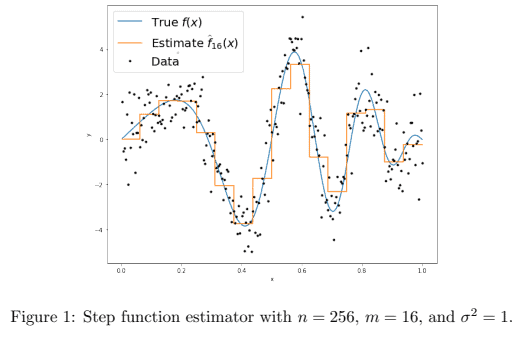
For $i=1, \ldots, n$ let $x_i=i / n$ and $y_i=f\left(x_i\right)+\epsilon_i$ where $\epsilon_i \sim \mathcal{N}\left(0, \sigma^2\right)$ for some unknown $f$ we wish to approximate at values $\left{x_i\right}_{i=1}^n$. We will approximate $f$ with a step function estimator. For some $m \leq n$ such that $n / m$ is an integer define the estimator
$$
\widehat{f}m(x)=\sum{j=1}^{n / m} c_j \mathbf{1}\left{x \in\left(\frac{(j-1) m}{n}, \frac{j m}{n}\right]\right} \quad \text { where } \quad c_j=\frac{1}{m} \sum_{i=(j-1) m+1}^{j m} y_i .
$$
Note that this estimator just partitions ${1, \ldots, n}$ into intervals ${1, \ldots, m},{m+1, \ldots, 2 m}, \ldots,{n-m+$ $1, \ldots, n}$ and predicts the average of the observations within each interval (see Figure 1 ).
By the bias-variance decomposition at some $x_i$ we have
$$
\mathbb{E}\left[\left(\widehat{f}m\left(x_i\right)-f\left(x_i\right)\right)^2\right]=\underbrace{\left(\mathbb{E}\left[\widehat{f}_m\left(x_i\right)\right]-f\left(x_i\right)\right)^2}{\operatorname{Bias}^2\left(x_i\right)}+\underbrace{\mathbb{E}\left[\left(\widehat{f}m\left(x_i\right)-\mathbb{E}\left[\widehat{f}_m\left(x_i\right)\right]\right)^2\right]}{\text {Variance }\left(x_i\right)}
$$

a. 5 points Intuitively, how do you expect the bias and variance to behave for small values of $m$ ? What about large values of $m$ ?
b. 5 points If we define $\bar{f}^{(j)}=\frac{1}{m} \sum_{i=(j-1) m+1}^{j m} f\left(x_i\right)$ and the average bias-squared as $\frac{1}{n} \sum_{i=1}^n\left(\mathbb{E}\left[\widehat{f}m\left(x_i\right)\right]-\right.$ $\left.f\left(x_i\right)\right)^2$, show that $$ \frac{1}{n} \sum{i=1}^n\left(\mathbb{E}\left[\widehat{f}m\left(x_i\right)\right]-f\left(x_i\right)\right)^2=\frac{1}{n} \sum{j=1}^{n / m} \sum_{i=(j-1) m+1}^{j m}\left(\bar{f}^{(j)}-f\left(x_i\right)\right)^2
$$
c. $\left[5\right.$ points] If we define the average variance as $\mathbb{E}\left[\frac{1}{n} \sum_{i=1}^n\left(\widehat{f}m\left(x_i\right)-\mathbb{E}\left[\widehat{f}_m\left(x_i\right)\right]\right)^2\right]$, show (both equalities) $$ \mathbb{E}\left[\frac{1}{n} \sum{i=1}^n\left(\widehat{f}m\left(x_i\right)-\mathbb{E}\left[\widehat{f}_m\left(x_i\right)\right]\right)^2\right]=\frac{1}{n} \sum{j=1}^{n / m} m \mathbb{E}\left[\left(c_j-\bar{f}^{(j)}\right)^2\right]=\frac{\sigma^2}{m}
$$
d. 15 points Let $n=256, \sigma^2=1$, and $f(x)=4 \sin (\pi x) \cos \left(6 \pi x^2\right)$. For values of $m=1,2,4,8,16,32$ plot the average empirical error $\frac{1}{n} \sum_{i=1}^n\left(\widehat{f}m\left(x_i\right)-f\left(x_i\right)\right)^2$ using randomly drawn data as a function of $m$ on the $x$-axis. On the same plot, using parts $\mathrm{b}$ and $\mathrm{c}$ of above, plot the average bias-squared, the average variance, and their sum (the average error). Thus, there should be 4 lines on your plot, each described in a legend. e. (Extra credit $[5$ points $]$ ) By the Mean-Value theorem we have that $\min {i=(j-1) m+1, \ldots, j m} f\left(x_i\right) \leq \bar{f}^{(j)} \leq$ $\max _{i=(j-1) m+1, \ldots, j m} f\left(x_i\right)$. Suppose $f$ is $L$-Lipschitz so that $\left|f\left(x_i\right)-f\left(x_j\right)\right| \leq \frac{L}{n}|i-j|$ for all $i, j \in{1, \ldots, n}$ for some $L<0$. Show that the average bias-squared is $O\left(\frac{L^2 m^2}{n^2}\right)$. Using the expression for average variance above, the total error behaves like $O\left(\frac{L^2 m^2}{n^2}+\frac{1}{m}\right)$. Minimize this expression with respect to $m$. Does this value of $m$, and the total error when you plug this value of $m$ back in, behave in an intuitive way with respect to $n, L, \sigma^2$ ? It turns out that this simple estimator (with the optimized choice of $m$ ) obtains the best achievable error rate up to a universal constant in this setup for this class of $L$-Lipschitz functions (see Tsybakov’s Introduction to Nonparametric Estimation for details).

This setup of each $x_i$ deterministically placed at $i / n$ is a good approximation for the more natural setting where each $x_i$ is drawn uniformly at random from $[0,1]$. In fact, one can redo this problem and obtain nearly identical conclusions, but the calculations are messier.