MY-ASSIGNMENTEXPERT™可以为您提供 lse.ac.uk ST227 Survival Models 生存模型的代写代考和辅导服务!
这是伦敦政经学院 生存模型课程的代写成功案例。
ST227课程简介
This course is compulsory on the BSc in Actuarial Science. This course is available on the BSc in Business Mathematics and Statistics, BSc in Data Science and BSc in Mathematics, Statistics and Business. This course is available as an outside option to students on other programmes where regulations permit and to General Course students.
Students must have completed Mathematical Methods (MA100) and Elementary Statistical Theory (ST102).
“Students must have completed one of the following two combinations of courses: (a) ST102 and MA100, or (b) MA107 and ST109 and EC1C1. Equivalent combinations may be accepted at the lecturer’s discretion.”
Prerequisites
An introduction to stochastic processes with emphasis on life history analysis and actuarial applications. Principles of modelling; model selection, calibration, and testing; Stochastic processes and their classification into different types by time space, state space, and distributional properties; construction of stochastic processes from finite-dimensional distributions, processes with independent increments, Poisson processes and renewal processes and their applications in general insurance and risk theory, Markov processes, Markov chains and their applications in life insurance and general insurance, extensions to more general intensity-driven processes, counting processes, semi-Markov processes, stationary distributions. Determining transition probabilities and other conditional probabilities and expected values; Integral expressions, Kolmogorov differential equations, numerical solutions, simulation techniques.
ST227 Survival Models HELP(EXAM HELP, ONLINE TUTOR)
The file Canada-mortality.txt (on the course web site) contains age-specific mortality rates $q_x$ for Canadian females and males for 2009-2011. Using the function lifeTable in the file survival-analysis. R (also on the web site), compute life tables for females and males.
(a) Compare the expectation of life at birth for females and males.
(b) Graph and compare the age-specific mortality rates $q_x$ for females and males.
(c) Graph and compare the numbers of survivors by age $l_x$ from the life tables for females and males. Suggestions: Use log vertical axes for these graphs; note that you can add a line to an existing graph with the lines function in $\mathrm{R}$ (see the R script from the lecture for examples).
The file Henning.txt (on the course web site) contains data from yet another study of criminal recidivism, this one by Henning and Frueh (1996), who followed 194 inmates released from a medium-security prison to a maximum of 3 years from the day of their release; during the period of the study, 106 of the released prisoners were rearrested (depressing, eh?). The data set, which is discussed by Judith Singer and John Willet in Applied Longitudinal Data Analysis (Oxford, 2003), contains the following variables (using the names employed by Singer and Willet):
- months: The time of re-arrest in months (but measured to the nearest day).
- censor: A dummy variable coded 1 for censored observations and 0 for uncensored observations. Note that this is the opposite of our usual convention, so in $\mathrm{R}$ survival time and censoring should be specified as Surv (months, censor $==0$ ); be careful to use the double-equals sign for testing equality!
- personal: A dummy variable coded 1 for prisoners with a record of crime against persons and 0 otherwise.
- property: A dummy variable coded 1 for prisoners with a record of crime against property and 0 otherwise.
- cage: “Centered” age in years at time of release – that is, age – average age.
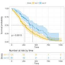
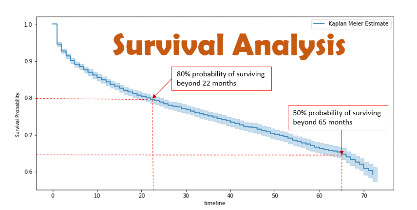
(a) Compute and graph the Kaplan-Meier estimate of the survival function for all of the data.
(b) Compute and graph separate survival curves for those with and without a record of crime against persons; test for differences between the two survival functions.
(c) Compute and graph separate survival curves for those with and without a record of crime against property; test for differences between the two survival functions.
Continuing with the Henning and Frueh data, fit a Cox regression of time to re-arrest on the covariates personal, property, and cage.
(a) Determine by a Wald test whether each estimated coefficient is statistically significant.
(b) Interpret each of the estimated Cox-regression coefficients.
Now consider the possibility that personal and property interact in determining time of re-arrest, by specifying the model formula Surv (months, censor == 0) personal*property + cage. Test the statistical significiance of the interaction in two ways: (1) by a Wald test of the coefficient for the interaction regressor personal:property; and (2) by a partial-likelihood-ratio test.
You can use the generic anova function to perform the likelihood-ratio test: Assuming that the two fitted models are named mod. 1 and mod. 2, the partial-likelihood-ratio test is obtained by anova (mod. 1 , mod.2, test=”Chisq”)
Are the results of the Wald and likelihood-ratio tests similar? What do you conclude about the interaction between personal and property?

MY-ASSIGNMENTEXPERT™可以为您提供 LSE.AC.UK ST227 SURVIVAL MODELS 生存模型的代写代考和辅导服务!