如果你也在 怎样代写最优化Optimization Theory 这个学科遇到相关的难题,请随时右上角联系我们的24/7代写客服。最优化Optimization Theory是致力于解决优化问题的数学分支。 优化问题是我们想要最小化或最大化函数值的数学函数。 这些类型的问题在计算机科学和应用数学中大量存在。
最优化Optimization Theory每个优化问题都包含三个组成部分:目标函数、决策变量和约束。 当人们谈论制定优化问题时,它意味着将“现实世界”问题转化为包含这三个组成部分的数学方程和变量。目标函数,通常表示为 f 或 z,反映要最大化或最小化的单个量。交通领域的例子包括“最小化拥堵”、“最大化安全”、“最大化可达性”、“最小化成本”、“最大化路面质量”、“最小化排放”、“最大化收入”等等。
最优化Optimization Theory代写,免费提交作业要求, 满意后付款,成绩80\%以下全额退款,安全省心无顾虑。专业硕 博写手团队,所有订单可靠准时,保证 100% 原创。最高质量的最优化Optimization Theory作业代写,服务覆盖北美、欧洲、澳洲等 国家。 在代写价格方面,考虑到同学们的经济条件,在保障代写质量的前提下,我们为客户提供最合理的价格。 由于作业种类很多,同时其中的大部分作业在字数上都没有具体要求,因此最优化Optimization Theory作业代写的价格不固定。通常在专家查看完作业要求之后会给出报价。作业难度和截止日期对价格也有很大的影响。
同学们在留学期间,都对各式各样的作业考试很是头疼,如果你无从下手,不如考虑my-assignmentexpert™!
my-assignmentexpert™提供最专业的一站式服务:Essay代写,Dissertation代写,Assignment代写,Paper代写,Proposal代写,Proposal代写,Literature Review代写,Online Course,Exam代考等等。my-assignmentexpert™专注为留学生提供Essay代写服务,拥有各个专业的博硕教师团队帮您代写,免费修改及辅导,保证成果完成的效率和质量。同时有多家检测平台帐号,包括Turnitin高级账户,检测论文不会留痕,写好后检测修改,放心可靠,经得起任何考验!
想知道您作业确定的价格吗? 免费下单以相关学科的专家能了解具体的要求之后在1-3个小时就提出价格。专家的 报价比上列的价格能便宜好几倍。
数学代写|最优化作业代写optimization theory代考|Why Use State Variables?
Having the mathematical model in state variable form is convenient because
The differential equations are ideally suited for digital or analog solution.
The state form provides a unified framework for the study of nonlinear and linear systems.
The state variable form is invaluable in theoretical investigations.
The concept of state has strong physical motivation.
Definition of State of a System
When referring to the state of a system, we shall have the following definition in mind.
DEFINITION 1-7
The state of a system is a set of quantities $x_1(t), x_2(t), \ldots, x_n(t)$
which if known at $t=t_0$ are determined for $t \geq t_0$ by specifying the inputs to the system for $t \geq t_0$.
System Classification
Systems are described by the terms linear, nonlinear, time-invariant, $\dagger$ and time-varying. We shall classify systems according to the form of their state equations. For example, if a system is nonlinear and time-varying, the state equations are written
$$
\dot{\mathbf{x}}(t)=\mathbf{a}(\mathbf{x}(t), \mathbf{u}(t), t) .
$$
Nonlinear, time-invariant systems are represented by state equations of the form
$$
\dot{\mathbf{x}}(t)=\mathbf{a}(\mathbf{x}(t), \mathbf{u}(t))
$$
If a system is linear and time-varying its state equations are
$$
\dot{\mathbf{x}}(t)=\mathbf{A}(t) \mathbf{x}(t)+\mathbf{B}(t) \mathbf{u}(t),
$$
where $\mathbf{A}(t)$ and $\mathbf{B}(t)$ are $n \times n$ and $n \times m$ matrices with time-varying elements. State equations for linear, time-invariant systems have the form
$$
\dot{\mathbf{x}}(t)=\mathbf{A} \mathbf{x}(t)+\mathbf{B u}(t)
$$
where $\mathbf{A}$ and $\mathbf{B}$ are constant matrices.
数学代写|最优化作业代写optimization theory代考|Output Equations
The physical quantities that can be measured are called the outputs and are denoted by $y_1(t), y_2(t), \ldots, y_q(t)$. If the outputs are nonlinear, time-varying functions of the states and controls, we write the output equations
$$
\mathbf{y}(t)=\mathbf{c}(\mathbf{x}(t), \mathbf{u}(t), t)
$$
If the output is related to the states and controls by a linear, time-invariant relationship, then
$$
\mathbf{y}(t)=\mathbf{C x}(t)+\mathbf{D u}(t)
$$
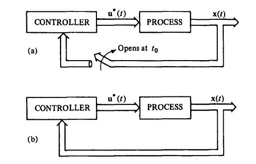
where $\mathbf{C}$ and $\mathbf{D}$ are $q \times n$ and $q \times m$ constant matrices. A nonlinear, timevarying system and a linear, time-invariant system are shown in Fig. 1-9. $\mathbf{r}(t)$, which has not been included in the state equations and represents any inputs that are not controlled, is called the reference or command input.
In our discussion of optimal control theory we shall make the simplifying assumption that the states are all available for measurement; that is, $\mathbf{y}(t)=\mathbf{x}(t)$
Solution of the State Equations-Linear Systems
For linear systems the state equations $(1.2-3)$ have the solution
$$
\mathbf{x}(t)=\varphi\left(t, t_0\right) \mathbf{x}\left(t_0\right)+\int_{t_0}^t \varphi(t, \tau) \mathbf{B}(\tau) \mathbf{u}(\tau) d \tau
$$
where $\varphi\left(t, t_0\right)$ is the state transition matrixt of the system. If the system is time-invariant as well as linear, $t_0$ can be set equal to 0 and the solution of the state equations is given by any of the three equivalent forms
$$
\begin{aligned}
& \mathbf{x}(t)=\mathscr{L}^{-1}\left{[s \mathbf{I}-\mathbf{A}]^{-1} \mathbf{x}(0)+[s \mathbf{I}-\mathbf{A}]^{-1} \mathbf{B U}(s)\right} \
& \mathbf{x}(t)=\mathscr{L}^{-1}{\boldsymbol{\Phi}(s) \mathbf{x}(0)+\mathbf{H}(s) \mathbf{U}(s)} \
& \mathbf{x}(t)=\epsilon^{\mathbf{A} t} \mathbf{x}(0)+\epsilon^{\mathbf{A} t} \int_0^t \epsilon^{-\mathbf{A \tau}} \mathbf{B u}(\tau) d \tau
\end{aligned}
$$
where $\mathbf{U}(s)$ and $\Phi(s)$ are the Laplace transforms of $\mathbf{u}(t)$ and $\boldsymbol{\varphi}(t), \mathscr{L}^{-1}{\cdot}$ denotes the inverse Laplace transform of ${\cdot}$, and $\epsilon^{\mathbf{A t}}$ is the $n \times n$ matrix
$$
\boldsymbol{\epsilon}^{\mathbf{A} t} \triangleq \mathbf{I}+\mathbf{A} t+\frac{1}{2 !} \mathbf{A}^2 t^2+\frac{1}{3 !} \mathbf{A}^3 t^3+\cdots+\frac{1}{k !} \mathbf{A}^k t^k+\cdots
$$
最优化代写
数学代写|最优化作业代写optimization theory代考|Why Use State Variables?
状态变量形式的数学模型是方便的,因为
微分方程非常适合数字或模拟解。
状态形式为研究非线性和线性系统提供了一个统一的框架。
状态变量形式在理论研究中是非常宝贵的。
状态的概念具有很强的物理动机。
系统状态的定义
当提到系统的状态时,我们应该记住下面的定义。
定义1-7
系统的状态是一组量$x_1(t), x_2(t), \ldots, x_n(t)$
,如果这些量在$t=t_0$已知,则通过指定系统在$t \geq t_0$的输入来确定$t \geq t_0$。
系统分类
系统用以下术语描述:线性、非线性、时不变、$\dagger$和时变。我们将根据状态方程的形式对系统进行分类。例如,如果一个系统是非线性时变的,状态方程写成
$$
\dot{\mathbf{x}}(t)=\mathbf{a}(\mathbf{x}(t), \mathbf{u}(t), t) .
$$
非线性时不变系统用
$$
\dot{\mathbf{x}}(t)=\mathbf{a}(\mathbf{x}(t), \mathbf{u}(t))
$$
形式的状态方程表示。如果一个系统是线性时变的,其状态方程为
$$
\dot{\mathbf{x}}(t)=\mathbf{A}(t) \mathbf{x}(t)+\mathbf{B}(t) \mathbf{u}(t),
$$
,其中$\mathbf{A}(t)$和$\mathbf{B}(t)$分别是具有时变元素的$n \times n$和$n \times m$矩阵。线性定常系统的状态方程形式为
$$
\dot{\mathbf{x}}(t)=\mathbf{A} \mathbf{x}(t)+\mathbf{B u}(t)
$$
,其中$\mathbf{A}$和$\mathbf{B}$是常数矩阵。
数学代写|最优化作业代写optimization theory代考|Output Equations
可以测量的物理量称为输出,用$y_1(t), y_2(t), \ldots, y_q(t)$表示。如果输出是状态和控制的非线性时变函数,我们写出输出方程
$$
\mathbf{y}(t)=\mathbf{c}(\mathbf{x}(t), \mathbf{u}(t), t)
$$
如果输出与状态和控制通过线性时不变关系相关,则
$$
\mathbf{y}(t)=\mathbf{C x}(t)+\mathbf{D u}(t)
$$
其中$\mathbf{C}$和$\mathbf{D}$是$q \times n$和$q \times m$常数矩阵。一个非线性时变系统和一个线性时不变系统如图1-9所示。$\mathbf{r}(t)$没有包含在状态方程中,它表示任何不受控制的输入,它被称为参考或命令输入。
在我们讨论最优控制理论时,我们将做一个简化的假设,即所有状态都可用于测量;即$\mathbf{y}(t)=\mathbf{x}(t)$
状态方程的解——线性系统
对于线性系统,状态方程$(1.2-3)$有解
$$
\mathbf{x}(t)=\varphi\left(t, t_0\right) \mathbf{x}\left(t_0\right)+\int_{t_0}^t \varphi(t, \tau) \mathbf{B}(\tau) \mathbf{u}(\tau) d \tau
$$
,其中$\varphi\left(t, t_0\right)$为系统的状态转移矩阵。如果系统是时不变线性的,则$t_0$可设为0,状态方程的解可由以下三种等价形式中的任意一种给出
$$
\begin{aligned}
& \mathbf{x}(t)=\mathscr{L}^{-1}\left{[s \mathbf{I}-\mathbf{A}]^{-1} \mathbf{x}(0)+[s \mathbf{I}-\mathbf{A}]^{-1} \mathbf{B U}(s)\right} \
& \mathbf{x}(t)=\mathscr{L}^{-1}{\boldsymbol{\Phi}(s) \mathbf{x}(0)+\mathbf{H}(s) \mathbf{U}(s)} \
& \mathbf{x}(t)=\epsilon^{\mathbf{A} t} \mathbf{x}(0)+\epsilon^{\mathbf{A} t} \int_0^t \epsilon^{-\mathbf{A \tau}} \mathbf{B u}(\tau) d \tau
\end{aligned}
$$
其中$\mathbf{U}(s)$和$\Phi(s)$为$\mathbf{u}(t)$的拉普拉斯变换,$\boldsymbol{\varphi}(t), \mathscr{L}^{-1}{\cdot}$为${\cdot}$的拉普拉斯逆变换,$\epsilon^{\mathbf{A t}}$为$n \times n$矩阵
$$
\boldsymbol{\epsilon}^{\mathbf{A} t} \triangleq \mathbf{I}+\mathbf{A} t+\frac{1}{2 !} \mathbf{A}^2 t^2+\frac{1}{3 !} \mathbf{A}^3 t^3+\cdots+\frac{1}{k !} \mathbf{A}^k t^k+\cdots
$$

数学代写|最优化作业代写optimization theory代考 请认准UprivateTA™. UprivateTA™为您的留学生涯保驾护航。
微观经济学代写
微观经济学是主流经济学的一个分支,研究个人和企业在做出有关稀缺资源分配的决策时的行为以及这些个人和企业之间的相互作用。my-assignmentexpert™ 为您的留学生涯保驾护航 在数学Mathematics作业代写方面已经树立了自己的口碑, 保证靠谱, 高质且原创的数学Mathematics代写服务。我们的专家在图论代写Graph Theory代写方面经验极为丰富,各种图论代写Graph Theory相关的作业也就用不着 说。
线性代数代写
线性代数是数学的一个分支,涉及线性方程,如:线性图,如:以及它们在向量空间和通过矩阵的表示。线性代数是几乎所有数学领域的核心。
博弈论代写
现代博弈论始于约翰-冯-诺伊曼(John von Neumann)提出的两人零和博弈中的混合策略均衡的观点及其证明。冯-诺依曼的原始证明使用了关于连续映射到紧凑凸集的布劳威尔定点定理,这成为博弈论和数学经济学的标准方法。在他的论文之后,1944年,他与奥斯卡-莫根斯特恩(Oskar Morgenstern)共同撰写了《游戏和经济行为理论》一书,该书考虑了几个参与者的合作游戏。这本书的第二版提供了预期效用的公理理论,使数理统计学家和经济学家能够处理不确定性下的决策。
微积分代写
微积分,最初被称为无穷小微积分或 “无穷小的微积分”,是对连续变化的数学研究,就像几何学是对形状的研究,而代数是对算术运算的概括研究一样。
它有两个主要分支,微分和积分;微分涉及瞬时变化率和曲线的斜率,而积分涉及数量的累积,以及曲线下或曲线之间的面积。这两个分支通过微积分的基本定理相互联系,它们利用了无限序列和无限级数收敛到一个明确定义的极限的基本概念 。
计量经济学代写
什么是计量经济学?
计量经济学是统计学和数学模型的定量应用,使用数据来发展理论或测试经济学中的现有假设,并根据历史数据预测未来趋势。它对现实世界的数据进行统计试验,然后将结果与被测试的理论进行比较和对比。
根据你是对测试现有理论感兴趣,还是对利用现有数据在这些观察的基础上提出新的假设感兴趣,计量经济学可以细分为两大类:理论和应用。那些经常从事这种实践的人通常被称为计量经济学家。
Matlab代写
MATLAB 是一种用于技术计算的高性能语言。它将计算、可视化和编程集成在一个易于使用的环境中,其中问题和解决方案以熟悉的数学符号表示。典型用途包括:数学和计算算法开发建模、仿真和原型制作数据分析、探索和可视化科学和工程图形应用程序开发,包括图形用户界面构建MATLAB 是一个交互式系统,其基本数据元素是一个不需要维度的数组。这使您可以解决许多技术计算问题,尤其是那些具有矩阵和向量公式的问题,而只需用 C 或 Fortran 等标量非交互式语言编写程序所需的时间的一小部分。MATLAB 名称代表矩阵实验室。MATLAB 最初的编写目的是提供对由 LINPACK 和 EISPACK 项目开发的矩阵软件的轻松访问,这两个项目共同代表了矩阵计算软件的最新技术。MATLAB 经过多年的发展,得到了许多用户的投入。在大学环境中,它是数学、工程和科学入门和高级课程的标准教学工具。在工业领域,MATLAB 是高效研究、开发和分析的首选工具。MATLAB 具有一系列称为工具箱的特定于应用程序的解决方案。对于大多数 MATLAB 用户来说非常重要,工具箱允许您学习和应用专业技术。工具箱是 MATLAB 函数(M 文件)的综合集合,可扩展 MATLAB 环境以解决特定类别的问题。可用工具箱的领域包括信号处理、控制系统、神经网络、模糊逻辑、小波、仿真等。