
如果你也在 怎样代写微积分Calculus 这个学科遇到相关的难题,请随时右上角联系我们的24/7代写客服。微积分Calculus 最初被称为无穷小微积分或 “无穷小的微积分”,是对连续变化的数学研究,就像几何学是对形状的研究,而代数是对算术运算的概括研究一样。
微积分Calculus 它有两个主要分支,微分和积分;微分涉及瞬时变化率和曲线的斜率,而积分涉及数量的累积,以及曲线下或曲线之间的面积。这两个分支通过微积分的基本定理相互关联,它们利用了无限序列和无限数列收敛到一个明确定义的极限的基本概念 。17世纪末,牛顿(Isaac Newton)和莱布尼兹(Gottfried Wilhelm Leibniz)独立开发了无限小数微积分。后来的工作,包括对极限概念的编纂,将这些发展置于更坚实的概念基础上。今天,微积分在科学、工程和社会科学中得到了广泛的应用。
微积分Calculus 代写,免费提交作业要求, 满意后付款,成绩80\%以下全额退款,安全省心无顾虑。专业硕 博写手团队,所有订单可靠准时,保证 100% 原创。 最高质量的微积分Calculus 作业代写,服务覆盖北美、欧洲、澳洲等 国家。 在代写价格方面,考虑到同学们的经济条件,在保障代写质量的前提下,我们为客户提供最合理的价格。 由于作业种类很多,同时其中的大部分作业在字数上都没有具体要求,因此微积分Calculus 作业代写的价格不固定。通常在专家查看完作业要求之后会给出报价。作业难度和截止日期对价格也有很大的影响。
同学们在留学期间,都对各式各样的作业考试很是头疼,如果你无从下手,不如考虑my-assignmentexpert™!
my-assignmentexpert™提供最专业的一站式服务:Essay代写,Dissertation代写,Assignment代写,Paper代写,Proposal代写,Proposal代写,Literature Review代写,Online Course,Exam代考等等。my-assignmentexpert™专注为留学生提供Essay代写服务,拥有各个专业的博硕教师团队帮您代写,免费修改及辅导,保证成果完成的效率和质量。同时有多家检测平台帐号,包括Turnitin高级账户,检测论文不会留痕,写好后检测修改,放心可靠,经得起任何考验!
想知道您作业确定的价格吗? 免费下单以相关学科的专家能了解具体的要求之后在1-3个小时就提出价格。专家的 报价比上列的价格能便宜好几倍。
我们在数学Mathematics代写方面已经树立了自己的口碑, 保证靠谱, 高质且原创的数学Mathematics代写服务。我们的专家在微积分Calculus Assignment代写方面经验极为丰富,各种微积分Calculus Assignment相关的作业也就用不着 说。
数学代写|微积分代写Calculus代考|Acceleration
Let’s go over acceleration: Put your pedal to the metal.
Positive and negative acceleration
The graph of the acceleration function at the bottom of Figure 7-2 is a simple line, $A(t)=6 t-12$. It’s easy to see that the acceleration of the yo-yo goes from a minimum of $-12 \frac{\text { inches per second }}{\text { second }}$ at $t=0$ seconds to a maximum of $12 \frac{\text { inches per second }}{\text { second }}$ at $t=4$ seconds, and that the acceleration is zero at $t=2$ when the yo-yo reaches its minimum velocity (and maximum speed). When the acceleration is negative – on the interval $[0,2)$ – that means that the velocity is decreasing. When the acceleration is positive – on the interval $(2,4]$ – the velocity is increasing.
Speeding up and slowing down
Figuring out when the yo-yo is speeding up and slowing down is probably more interesting and descriptive of its motion than the info in the preceding section. An object is speeding up (what we call “acceleration” in everyday speech) whenever the velocity and the calculus acceleration are both positive or both negative. And an object is slowing down (what we call “deceleration”) when the velocity and the calculus acceleration are of opposite signs.
Look at all three graphs in Figure 7-2 again. From $t=0$ to about $t=0.47$ (when velocity is zero), the velocity is positive and the acceleration is negative, so the yo-yo is slowing down (till it reaches its maximum height). When $t=0$, the deceleration is greatest (12 $\frac{\text { inches per second }}{\text { second }}$; the graph shows negative 12, but I’m calling it positive 12 because I’m calling it a deceleration, get it?) From about $t=0.47$ to $t=2$, both velocity and acceleration are negative, so the yo-yo is speeding up. From $t=2$ to about $t=3.53$, velocity is positive and acceleration is negative, so the yo-yo is slowing down again (till it bottoms out at its lowest height). Finally, from about $t=3.53$ to $t=4$, both velocity and acceleration are positive, so the yo-yo is speeding up again. The yo-yo reaches its greatest acceleration of $12 \frac{\text { inches per second }}{\text { second }}$ at $t=4$ seconds.
Tying it all together
Note the following connections among the three graphs in Figure 7-2. The negative section on the graph of $A(t)-$ from $t=0$ to $t=2-$ corresponds to a decreasing section of the graph of $V(t)$ and a concave down section of the graph of $H(t)$. The positive interval on the graph of $A(t)-$ from $t=2$ to $t=4-$ corresponds to an increasing interval on the graph of $V(t)$ and a concave up interval on the graph of $H(t)$. When $t=2$ seconds, $A(t)$ has a zero, $V(t)$ has a local minimum, and $H(t)$ has an inflection point.
数学代写|微积分代写Calculus代考|Related Rates
Say you’re filling up your swimming pool; you know how fast water is coming out of your hose, and you want to calculate how fast the water level in the pool is rising. You know one rate (how fast the water is pouring in), and you want to determine another rate (how fast the water level is rising). These rates are called related rates because one depends on the other – the faster the water is poured in, the faster the water level rises. In a typical related rates problem, the rate or rates you’re given are unchanging, but the rate you have to figure out is changing with time. You have to determine this rate at one particular point in time.
A calculus crossroads
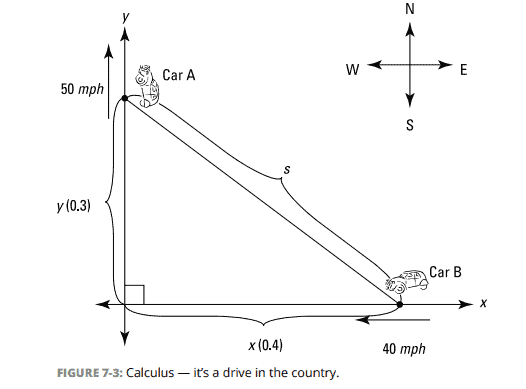
One car leaves an intersection traveling north at $50 \mathrm{mph}$; another is driving west toward the intersection at $40 \mathrm{mph}$. At one point, the north-bound car is three-tenths of a mile north of the intersection and the west-bound car is four-tenths of a mile east of it. At this point, how fast is the distance between the cars changing?
Draw a diagram and label it with any unchanging measurements (there are none in this particular problem), and make sure to assign a variable to anything in the problem that’s changing (unless it’s irrelevant to the problem). See Figure 7-3.
Note that variables have been assigned to the distance between Car A and the intersection, the distance between $\mathrm{Car} \mathrm{B}$ and the intersection, and the distance between the two cars, because those are changing distances. The 0.3 and 0.4 are in parentheses to emphasize that theyre not unchanging measurements; they’re the distances at one particular point in time.
In related rates problems, it’s important to distinguish between what is changing and what is not changing.
You may run across a similar problem in your calculus textbook. It involves a ladder leaning against and sliding down a wall. The diagram for this problem would be very similar to Figure 7-3 except that the $y$-axis would represent the wall, the $x$-axis would be the ground, and the diagonal line would be the ladder. Despite the similarities between these two problems, there’s an important difference: The distance between the cars is changing, so the diagonal line in Figure 7-3 is labeled with a variable, s. A ladder, on the other hand, has a fixed length, so the diagonal line in the diagram for the ladder problem would be labeled with a number, not a variable.
微积分代写
数学代写|微积分代写Calculus代考|Acceleration
让我们来复习一下加速:把你的踏板踩到金属上。
正负加速度
图7-2底部的加速度函数曲线图是一条简单的线,$ a (t)=6 t-12$。很容易看出,溜溜球的加速度从$t=0$秒时的最小值$-12 \frac{\text {second}}$到$t=4$秒时的最大值$12 \frac{\text {seconds}$,当溜溜球达到最小速度(和最大速度)时,加速度为$t=2$为零。当加速度为负时-在区间$[0,2)$上-这意味着速度在减小。当加速度为正时——在区间$(2,4]$上——速度在增加。
加速和减速
弄清楚溜溜球何时加速和减速可能比前一节的信息更有趣,更能描述它的运动。当速度和微积分加速度都为正或都为负时,物体就在加速(我们在日常用语中称之为“加速度”)。当速度和微积分加速度的符号相反时,物体就会减速(我们称之为“减速”)。再看一遍图7-2中的三个图。从$t=0$到$t=0.47$(当速度为零时),速度为正,加速度为负,因此溜溜球正在减速(直到达到最大高度)。当$t=0$时,减速最大(12 $\frac{\text{英寸/秒}}{\text{秒}}$;图形显示的是- 12,但我称它为正12因为我称它为减速,明白吗?)从约$t=0.47$到$t=2$,速度和加速度都是负的,所以溜溜球在加速。从$t=2$到$t=3.53$,速度为正,加速度为负,所以溜溜球再次减速(直到它在最低高度触底)。最后,从$t=3.53$到$t=4$,速度和加速度都是正的,所以溜溜球又加速了。在$t=4$秒时,溜溜球达到最大加速度$12 \frac{\text{英寸每秒}}{\text{秒}}$。
将它们结合在一起
请注意图7-2中三个图形之间的联系。$A(t)-$从$t=0$到$t=2-$图上的负截面对应于$V(t)$图的递减截面和$H(t)$图的下凹截面。$A(t)-$图上从$t=2$到$t=4-$的正区间对应于$V(t)$图上的递增区间和$H(t)$图上的上凹区间。当$t=2$秒时,$A(t)$有一个零点,$V(t)$有一个局部极小值,$H(t)$有一个拐点。
数学代写|微积分代写Calculus代考|Related Rates
比方说,你在给游泳池注满水;你知道水从水管流出的速度,你想计算池中的水位上升的速度。你知道一个速率(水涌入的速度),你想确定另一个速率(水位上升的速度)。这些速率被称为相关速率,因为一个速率依赖于另一个速率——水注入得越快,水位上升得越快。在典型的相关速率问题中,给定的速率是不变的,但是你要算出的速率是随时间变化的。你必须确定在某一特定时间点的速率。
微积分十字路口
一辆汽车以$50 \ mathm {mph}$的速度离开十字路口向北行驶;另一个正以每小时40美元的速度向西驶向十字路口。在某一时刻,向北行驶的汽车在十字路口以北十分之三英里处,向西行驶的汽车在十字路口以东十分之四英里处。在这一点,两车之间的距离变化有多快?
绘制一个图表,用任何不变的测量值标记它(在这个特定的问题中没有),并确保为问题中任何变化的东西分配一个变量(除非它与问题无关)。如图7-3所示。
注意,变量被赋值为汽车A到十字路口的距离,$\mathrm{Car} \mathrm{B}$到十字路口的距离,以及两辆车之间的距离,因为这些距离是变化的。0.3和0.4在括号中是为了强调它们不是不变的测量值;它们是在某一特定时间点的距离。
在相关的利率问题中,区分什么在变化,什么没有变化是很重要的。
你可能会在微积分课本上遇到类似的问题。它需要一个梯子靠在墙上,然后从墙上滑下来。这个问题的图表将与图7-3非常相似,除了y轴代表墙,x轴代表地面,对角线代表梯子。尽管这两个问题之间有相似之处,但有一个重要的区别:汽车之间的距离是变化的,所以图7-3中的对角线被标记为变量s。另一方面,梯子的长度是固定的,所以梯子问题图中的对角线将被标记为数字,而不是变量。

数学代写|微积分代写Calculus代考 请认准UprivateTA™. UprivateTA™为您的留学生涯保驾护航。
微观经济学代写
微观经济学是主流经济学的一个分支,研究个人和企业在做出有关稀缺资源分配的决策时的行为以及这些个人和企业之间的相互作用。my-assignmentexpert™ 为您的留学生涯保驾护航 在数学Mathematics作业代写方面已经树立了自己的口碑, 保证靠谱, 高质且原创的数学Mathematics代写服务。我们的专家在图论代写Graph Theory代写方面经验极为丰富,各种图论代写Graph Theory相关的作业也就用不着 说。
线性代数代写
线性代数是数学的一个分支,涉及线性方程,如:线性图,如:以及它们在向量空间和通过矩阵的表示。线性代数是几乎所有数学领域的核心。
博弈论代写
现代博弈论始于约翰-冯-诺伊曼(John von Neumann)提出的两人零和博弈中的混合策略均衡的观点及其证明。冯-诺依曼的原始证明使用了关于连续映射到紧凑凸集的布劳威尔定点定理,这成为博弈论和数学经济学的标准方法。在他的论文之后,1944年,他与奥斯卡-莫根斯特恩(Oskar Morgenstern)共同撰写了《游戏和经济行为理论》一书,该书考虑了几个参与者的合作游戏。这本书的第二版提供了预期效用的公理理论,使数理统计学家和经济学家能够处理不确定性下的决策。
微积分代写
微积分,最初被称为无穷小微积分或 “无穷小的微积分”,是对连续变化的数学研究,就像几何学是对形状的研究,而代数是对算术运算的概括研究一样。
它有两个主要分支,微分和积分;微分涉及瞬时变化率和曲线的斜率,而积分涉及数量的累积,以及曲线下或曲线之间的面积。这两个分支通过微积分的基本定理相互联系,它们利用了无限序列和无限级数收敛到一个明确定义的极限的基本概念 。
计量经济学代写
什么是计量经济学?
计量经济学是统计学和数学模型的定量应用,使用数据来发展理论或测试经济学中的现有假设,并根据历史数据预测未来趋势。它对现实世界的数据进行统计试验,然后将结果与被测试的理论进行比较和对比。
根据你是对测试现有理论感兴趣,还是对利用现有数据在这些观察的基础上提出新的假设感兴趣,计量经济学可以细分为两大类:理论和应用。那些经常从事这种实践的人通常被称为计量经济学家。
Matlab代写
MATLAB 是一种用于技术计算的高性能语言。它将计算、可视化和编程集成在一个易于使用的环境中,其中问题和解决方案以熟悉的数学符号表示。典型用途包括:数学和计算算法开发建模、仿真和原型制作数据分析、探索和可视化科学和工程图形应用程序开发,包括图形用户界面构建MATLAB 是一个交互式系统,其基本数据元素是一个不需要维度的数组。这使您可以解决许多技术计算问题,尤其是那些具有矩阵和向量公式的问题,而只需用 C 或 Fortran 等标量非交互式语言编写程序所需的时间的一小部分。MATLAB 名称代表矩阵实验室。MATLAB 最初的编写目的是提供对由 LINPACK 和 EISPACK 项目开发的矩阵软件的轻松访问,这两个项目共同代表了矩阵计算软件的最新技术。MATLAB 经过多年的发展,得到了许多用户的投入。在大学环境中,它是数学、工程和科学入门和高级课程的标准教学工具。在工业领域,MATLAB 是高效研究、开发和分析的首选工具。MATLAB 具有一系列称为工具箱的特定于应用程序的解决方案。对于大多数 MATLAB 用户来说非常重要,工具箱允许您学习和应用专业技术。工具箱是 MATLAB 函数(M 文件)的综合集合,可扩展 MATLAB 环境以解决特定类别的问题。可用工具箱的领域包括信号处理、控制系统、神经网络、模糊逻辑、小波、仿真等。