MY-ASSIGNMENTEXPERT™可以为您提供 sydney STAT4025 Time series analysis时间序列分析的代写代考和辅导服务!
这是悉尼大学 时间序列分析的代写成功案例。
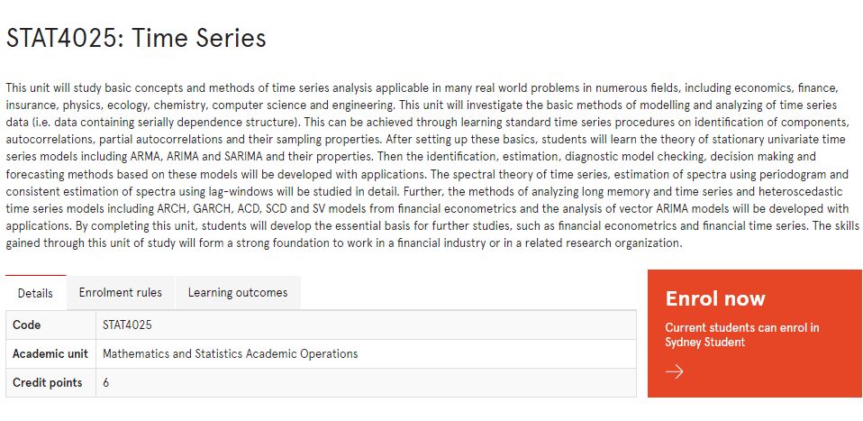
STAT4025课程简介
This unit will study basic concepts and methods of time series analysis applicable in many real world problems in numerous fields, including economics, finance, insurance, physics, ecology, chemistry, computer science and engineering. This unit will investigate the basic methods of modelling and analyzing of time series data (i.e. data containing serially dependence structure). This can be achieved through learning standard time series procedures on identification of components, autocorrelations, partial autocorrelations and their sampling properties. After setting up these basics, students will learn the theory of stationary univariate time series models including ARMA, ARIMA and SARIMA and their properties. Then the identification, estimation, diagnostic model checking, decision making and forecasting methods based on these models will be developed with applications. The spectral theory of time series, estimation of spectra using periodogram and consistent estimation of spectra using lag-windows will be studied in detail. Further, the methods of analyzing long memory and time series and heteroscedastic time series models including ARCH, GARCH, ACD, SCD and SV models from financial econometrics and the analysis of vector ARIMA models will be developed with applications. By completing this unit, students will develop the essential basis for further studies, such as financial econometrics and financial time series. The skills gained through this unit of study will form a strong foundation to work in a financial industry or in a related research organization.
Prerequisites
At the completion of this unit, you should be able to:
- LO1. 1. Explain and examine time series data and Identify components of a time series; remove trends, seasonal and other components.
- LO2. Identify stationarity time series; sample autocorrelations and partial autocorrelations, probability models for stationary time series.
- LO3. Explain homogeneous nonstationary time series, simple and integrated models and related results.
- LO4. Apply estimation and fitting methods for ARIMA models via MM and MLE methods. Apply hypothesis testing, diagnostic checking and goodness-of-fit tests
- LO5. Apply hypothesis testing, diagnostic checking and goodness-of-fit tests methodology.
- LO6. Construct forecasting methods for ARIMA models.
- LO7. Explain spectral methods in time series analysis
- LO8. Apply financial time series and related models to straightforward problems.
- LO9. Apply the methods of analysis of GARCH and other models for volatility.
- LO10. Explain and apply methods of vector time series models
STAT4025 Time series analysis HELP(EXAM HELP, ONLINE TUTOR)
As you read more of the time-series literature, you will find that different authors and different software packages report the AIC and the SBC (BIC) in various ways. The examples in Enders use
$$
\begin{aligned}
& A I C=T \log S S R+2 n \
& B I C=T \log S S R+n \log T
\end{aligned}
$$
where SSR = sum of squared residuals. EVIEWS, in general, uses the following
$$
\begin{aligned}
& A I C=-2 \log L / T+\frac{2 n}{T} \
& S B C=-2 \log L / T+\frac{n \log T}{T}
\end{aligned}
$$
where $L=$ maximised value of the likelihood function. Other sources use
$$
\begin{aligned}
A I C & =\frac{\exp (2 n / T) \cdot S S R}{T} \
B I C & =\frac{T^{n / T} S S R}{T}
\end{aligned}
$$
This is only an example of the different forms available. If you find this confusing you are correct. The problem is that some of the formulae are more convenient in certain circumstances. If you estimate one model with one piece of software and extract its AIC and then estimate a second model with a second piece of software and extract the AIC for the second model it is likely that the two estimates of AIC are not compatible. You will need to do a little more work. I have seen cases where a an econometric package used different versions of AIC for different estimation procedures but this was generally obvious.
(a) Show that all three methods of calculating the AIC will necessarily select the same model. [Hint: The AIC will select model 1 over model 2 if the AIC from model 1 is smaller than that from model 2. Show that all three ways of calculating the AIC are monotonic transformations of each other.]
(b) Show that all three methods of calculating the SBC will necessarily select the same model.
(c) Select one of the three pairs above. Show that the AIC will never select a more parsimonious model than the SBC.
The file QUARTERLY.XLS contains a number of series including the US index of industrial production (indprod), unemployment rate (urate) and producer price index for finished goods (finished). All the series run from 1960Q1 to 2008Q2.
(a) Exercise with indprod.
i. Construct the growth rate of the series as $y_t=\log$ indprod $_t-\log$ indprod $_{t-1}$. Since the first few autocorrelations suggest an AR(1) process, estimate $y_t=0.0035+0.543 y_{t-1}+$ $\varepsilon$ (the $t$-statistics are 3.50 and 9.02 respectively).
ii. Show that adding an MA term at lag 8 improves the fit and removes the serial correlation
(b) Exercise with urate
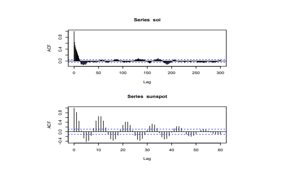
i. Examine the ACF of the series. It should be clear that the ACF decays slowly and that the PACF has a very negative spike at lag 2.
ii. Temporarily ignore the necessity of differencing the series. Estimate urate as an AR(2) process including a constant. You should find that $a_1+a_2=0.9980$
iii. Form the difference as $y_t=$ urate $_t-$ urate $_{t-1}$. Show that the model $y_t=\alpha_0+$ $\alpha_1 y_{t-1}+\beta_4 \varepsilon_{t-4}+\beta_8 \varepsilon_{t-8}+\varepsilon_t$ exhibits no remaining serial correlation and has a better fit than $y_t=\alpha_0+\alpha_1 y_{t-1}+\alpha_4 y_{t-4}+\beta_8 \varepsilon_{t-8}+\varepsilon_t$ or $y_t=\alpha_0+\alpha_1 y_{t-1}+\alpha_4 y_{t-4}+\alpha_8 y_{t-8}+\varepsilon_t$.
(c) Exercise with finished
i. Construct the growth rate of the series as $y_t=\log$ finished $-\log$ finished $_{t-1}$
ii. Show that an ARMA $(1,1)$ model fits the data well but that the residual autocorrelation at lag 3 is a problem.
iii. Show that an $\operatorname{ARMA}((1,3), 1)$ is not appropriate. Show that an $\operatorname{ARMA}(1,(1,3))$ shows no remaining residual correlation.
iv. Show that an $\mathrm{AR}(3)$ has the best fir and has no remaining serial correlation.
The file QUARTERLY.XLS contains the quarterly values of the Consumer Price Index (excluding food and fuel) that have not been seasonally adjusted(CPINSA). Form the inflation rate, as measured by the $C P I$ as $\ln \left(C P I N S A_t / C P I N S A_{t-1}\right)$
(a) Plot the inflation rate. Does there appear to be a plausible seasonal pattern in the data? Seasonally difference the CPI using $\Delta_4 \ln C P I N S A_t=\ln C P I N S A_t-\ln C P I N S A_{t-4}$ Find the ACF of this series and explain why it is not appropriate to apply Box-Jenkins methodology to this series
(b) For convenience let $\pi_t=(1-L)\left(1-L^4\right) \ln$ Cpinsa $a_t$. Find an appropriate model for the $\pi_t$ series. In particular consider the following four models for the series.
$$
\begin{array}{ll}
\pi_t=a_o+a_1 \pi_{t-1}+\varepsilon_t+\varepsilon_{t-4} & \text { Model 1: AR(1) with Seasonal MA } \
\pi_t=a_0+\left(1+a_1 L\right)\left(1+a_4 L \pi_{t-1}+\varepsilon_t\right. & \text { Model 2: Multiplicative Autoregressive } \
p i_t=a_0+\left(1+\beta_1 L\right)\left(1+\beta_4 L\right) \varepsilon_t & \text { Model 3: Multiplicative Moving Average } \
\pi_t=a_o+\left(a_1 \pi_{t-1}+\beta_1 \varepsilon t-1\right)\left(1+\beta_4 \varepsilon_{t-4}+\varepsilon_t\right. & \text { Model 4: ARMA(1,1) with Seasonal MA }
\end{array}
$$
Model 1: AR(1) with Seasonal MA
Model 2: Multiplicative Autoregressive
Model 3: Multiplicative Moving Average
Model 4: ARMA $(1,1)$ with Seasonal MA
The file labelled ARCH.csv contains the 100 realisations of the simulated $\left{y_t\right}$ sequence used to create the Panel (d) of Figure 3.7.(on page 129 of Enders (2010)). Recall that this series was simulated as $y_t=0.9 y_{t-1}+\varepsilon_t$, where $\varepsilon_t$ is the ARCH(1) error process $\varepsilon_t=v_t\left(1+0.8 \varepsilon_{t-1}\right)^{1 / 2}$. You should find the series has a mean of 0.263 , a standard deviation of 4.894 with minimum and maximum values of -10.8 and 15.15 , respectively.
(a) Estimate the series using OLS and save the residuals. You should obtain
$$
y_t=0.944 y_{t-1}+\varepsilon_t .
$$
The $t$-statistic for $\hat{\alpha}_1$ is 26.51 . Note that the estimated value of $\alpha_1$, differs from the theoretical value of 0.9 . This is due to nothing more than sampling error; the simulated values of $\left{v_t\right}$ do not precisely conform to the theoretical distribution. However, can you provide an intuitive explanation of why positive serial correlation in the $\left{v_t\right}$ sequence might shift the estimate of $\alpha_1$ upward in small samples?
(b) Obtain the ACF and the PACF of the residuals. Use LJung-Box Q-statistics to determine whether the residuals approximate white noise. You should find:
\begin{tabular}{ccccccccc}
& 1 & 2 & 3 & 4 & 5 & 6 & 7 & 8 \
\hline ACF & 0.149 & 0.004 & -0.018 & -0.012 & 0.068 & 0.003 & -0.099 & -0.151 \
PACF & 0.149 & -0.018 & -0.016 & -0.007 & 0.073 & -0.019 & -0.100 & -0.123 \
\hline
\end{tabular}
$$
Q(4)=2.31, Q(8)=6.39, Q(24)=18.49 \text {. }
$$
(c) Obtain the ACF and the PACF of the squared residuals. You should find:
\begin{tabular}{ccccccccc}
& 1 & 2 & 3 & 4 & 5 & 6 & 7 & 8 \
\hline ACF & 0.473 & 0.127 & -0.057 & -0.078 & 0.057 & 0.242 & 0.273 & 0.214 \
PACF & 0.474 & -0.125 & -0.086 & 0.004 & 0.135 & 0.198 & 0.070 & 0.062 \
\hline
\end{tabular}
Based on the ACF and PACF of the residuals and the squared residuals, what can you conclude about the presence of ARCH errors?
(d) Estimate the squared residuals as: $\varepsilon^2=\alpha_0+\alpha_1 \varepsilon_{t-1}^2$. You should verify that $\alpha_0=1.55$ $(t$-statistic $=2.83)$ and $\alpha_1=0.474$ (t-statistic $\left.=5.28\right)$
Show that the Lagrange multiplier ARCH(I) errors is: $T R^2=22.03$ with a significance level of 0.00000269 .
(e) Simultaneously estimate the $\left{y_t\right}$ sequence and the ARCH(I) error process using maximum likelihood estimation. You should find:
$$
\begin{aligned}
& y_t=0.886 \quad y_{t-1}+\varepsilon_t \quad h_t=1.16+0.663 \varepsilon_{t-1}^2 \
& \text { (33.00) } \
&
\end{aligned}
$$

MY-ASSIGNMENTEXPERT™可以为您提供 sydney STAT4025 Time series analysis时间序列分析的代写代考和辅导服务!