MY-ASSIGNMENTEXPERT™可以为您提供 sydney STAT4025 Time series analysis时间序列分析的代写代考和辅导服务!
这是悉尼大学 时间序列分析的代写成功案例。
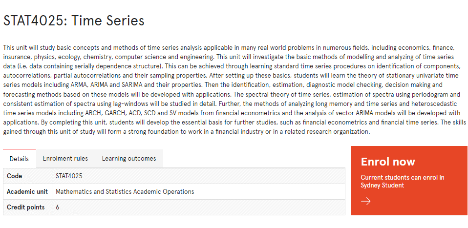
STAT4025课程简介
This unit will study basic concepts and methods of time series analysis applicable in many real world problems in numerous fields, including economics, finance, insurance, physics, ecology, chemistry, computer science and engineering. This unit will investigate the basic methods of modelling and analyzing of time series data (i.e. data containing serially dependence structure). This can be achieved through learning standard time series procedures on identification of components, autocorrelations, partial autocorrelations and their sampling properties. After setting up these basics, students will learn the theory of stationary univariate time series models including ARMA, ARIMA and SARIMA and their properties. Then the identification, estimation, diagnostic model checking, decision making and forecasting methods based on these models will be developed with applications. The spectral theory of time series, estimation of spectra using periodogram and consistent estimation of spectra using lag-windows will be studied in detail. Further, the methods of analyzing long memory and time series and heteroscedastic time series models including ARCH, GARCH, ACD, SCD and SV models from financial econometrics and the analysis of vector ARIMA models will be developed with applications. By completing this unit, students will develop the essential basis for further studies, such as financial econometrics and financial time series. The skills gained through this unit of study will form a strong foundation to work in a financial industry or in a related research organization.
Prerequisites
At the completion of this unit, you should be able to:
- LO1. 1. Explain and examine time series data and Identify components of a time series; remove trends, seasonal and other components.
- LO2. Identify stationarity time series; sample autocorrelations and partial autocorrelations, probability models for stationary time series.
- LO3. Explain homogeneous nonstationary time series, simple and integrated models and related results.
- LO4. Apply estimation and fitting methods for ARIMA models via MM and MLE methods. Apply hypothesis testing, diagnostic checking and goodness-of-fit tests
- LO5. Apply hypothesis testing, diagnostic checking and goodness-of-fit tests methodology.
- LO6. Construct forecasting methods for ARIMA models.
- LO7. Explain spectral methods in time series analysis
- LO8. Apply financial time series and related models to straightforward problems.
- LO9. Apply the methods of analysis of GARCH and other models for volatility.
- LO10. Explain and apply methods of vector time series models
STAT4025 Time series analysis HELP(EXAM HELP, ONLINE TUTOR)
The file ireland2.csv contains the total returns index for the ISEQ. (Total returns are calculated on the basis that dividends are reinvested).
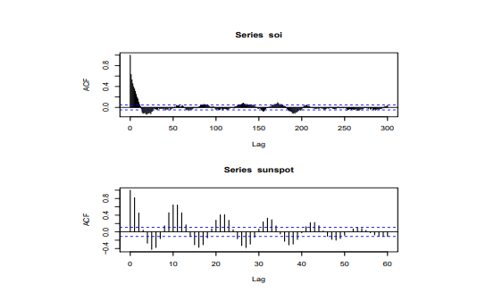
(a) Examine the series, ACF and PACF of the index in levels, first differences, logs and first differences of the logs. From an economic viewpoint which is the appropriate model for such a series. Does the data fit this viewpoint. Is there autocorrelation in the transformed series? Does this imply independence?
(b) Examine the squared values of the first differences of the logs and comment on the ACF and PACF of these first differences. Is there autocorrelation in this series. Comment on its relevance.
(c) Estimate an appropriate ARCH/GARCH model for the return series (First differences of logs)
The file cpi.csv contains data on the Irish CPI for the period 1957 Quarter 1 to 2006 Quarter 2. It also contains data on a variable $\mathrm{c}$ which has been proposed as an indicator of the level of the CPI. This indicator is exogenous, known in advance and can not be influenced by the authorities.
(a) Load the data into EVIEWS and add a EVIEWS date variable to the data set.
(b) Regress the log of the CPI on c and a constant and comment on the fit of the regression, $t$-statistics and the results of any specification tests that you consider appropriate. You should also examine the residuals from the regression. Using these results, is c a suitable predictor of the (log)CPI?
(c) An enquiry into the origin of c shows that it is cumulative rainfall in Armagh for the period 1857Q1 to $1906 \mathrm{Q} 2$. Is the apparent relationship due to chance or is there a deeper explanation for the spurious nature of the regression.
(d) List the kind of conclusions that can and can not be drawn from regression analysis with time series data
The data set npext.csv is an updated version of the Nelson-Plosser “unit root” data set and contains the fourteen U.S. economic time series set out below. All series are transformed by taking logarithms except for the bond yield. The sample period ends in 1988.
year Time index from 1860 until 1988.
realgn Real GNP, [Billions of 1958 Dollars, [1909 – 1988]
nomgnp Nominal GNP, [Millions of Current Dollars], [1909 – 1988]
gnpperca Real Per Capita GNP, [1958 Dollars], [1909 – 1988]
indprod Industrial Production Index, [1967 = 100], [1860 – 1988]
employmt Total Employment, [Thousands], [1890 – 1988]
unemploy Total Unemployment Rate, [Percent], [1890 – 1988]
gnpdefl GNP Deflator, [1958 = 100], [1889 – 1988]
cpi Consumer Price Index, [1967 = 100], [1860 – 1988]
wages Nominal Wages (Average annual earnings per full-time employee in manufacturing), [current Dollars], [1900 – 1988]
realwag Real Wages, [Nominal wages/CPI], [1900 – 1988]
M Money Stock (M2), [Billions of Dollars, annual averages], [1889 – 1988]
velocity Velocity of Money, [1869 – 1988]
interest Bond Yield (Basic Yields of 30-year corporate bonds), [Percent per annum], [1900 1988]
sp500 Stock Prices, [Index; 1941 – $43=100],[1871-1988]$
For a selected series
(a) Using graphs examine the series, it first difference, and whatever other transformations you consider necessary. Comment on what the graphs indicate.
(b) Does economics (or common sense) tell you if the variable is a random walk, a random walk with drift or a random walk with drift and trend. Do economics and the graphs agree. Which ADF test are you going to use?
(c) Choose a maximum lag order and then determine what is the appropriate lag length to use for an ADF or DF unit root test. (Use AIC, BIC and lag length reduction tests to determine the appropriate lag length).
(d) Implement an ADF test for the appropriate lag length (or range of lag lengths). Interpret your results. How sensitive are your conclusions to the choice of lag length?
(e) Implement an ERS test for a unit root. Compare the results of ADF and ERS tests
The file mypr3.csv contains the following series
obs Year of observation,
$m$ Logarithm of US M1,
$p$ Logarithm of Prices (Price Deflator for US Net National Product)
$y$ Logarithm of US real Net National Product
$r$ Interest Rates
$m r$ Logarithm of Real M1 $(m r=m-p)$
$\mathbf{v}$ Logarithm of Velocity $(v=y-m+p)$
Detailed definitions are in Appendix B of Stock and Watson (1993).4
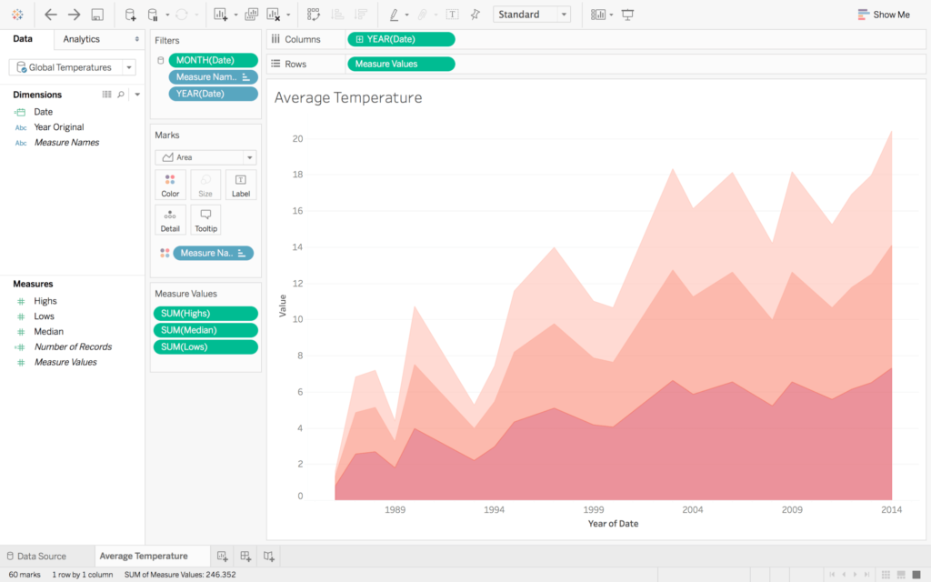
(a) Draw time series plots of
real Net National Product and Real M1
Log velocity and Interest Rates. Use separate axes for each variable.
Do these graphs provide any indication of a possible long run money demand function
(b) Complete Univariate Augmented Dickey-Fuller unit root tests for $m, m-p, y, r$, including 2 and 4 lags and report on your conclusions.
(c) Complete DF-GLS unit root test choosing SIC as criterion for number of lags to be included. Compare these results with those derived from the standard ADF tests.
(d) Test for co-integration of $m-p, y$ and $r$ using the Engle-Granger procedure. (There is no direct instruction in EVIEWS to complete this test. You must do the appropriate OLS estimate, save the residuals and then calculate the appropriate ADF test for the residuals. The critical values given by EVIEWS are for standard unit root tests and are not appropriate in this case. Correct Critical values are available in many textbooks. These critical values may depend on sample size and on number of variables (calculated in different ways in different tables). If you use the EVIEWS default (SIC) to determine the number of lags you will use two lags and reject co-integration. Stock and Watson (1993) use one lag and can not reject co-integration. Replicate and comment.
(e) Determine and appropriate lag-length for an appropriate VAR in the variables $m-p, y$ and $r$. You should find that you 1 or 2 lags is appropriate depending on the information criteria used. Do specification tests for a VAR with 2 lags.
(f) Do a Johansen test for co-integration in this VAR and determine an appropriate number of co-integrating vectors. Estimate the residuals in this VAR. Assuming one co-integrating relationship compare the results with the Engle-Granger results already obtained. Do these results provide evidence against a unit elasticity of real M1 with respect to income. Derive 95\% confidence intervals for the semi-elasticity of real M1 with respect to interest rates.
(g) Read the account of dynamic OLS (DOLS) in Stock and Watson (2007) or Hayashi (2000). This is a relatively simple way to estimate a long term relationship. Estimate a long run relationship between $m-p, y$ and $r$ using two lags and two leads of $\Delta y$ and $\delta r$. You should get and equation of the form
$$
\begin{array}{r}
m-p=0.970 y-0.101 r \
(.046) \quad(.013)
\end{array}
$$

MY-ASSIGNMENTEXPERT™可以为您提供 sydney STAT4025 Time series analysis时间序列分析的代写代考和辅导服务!