如果你也在 怎样代写运筹学Operations Research 这个学科遇到相关的难题,请随时右上角联系我们的24/7代写客服。运筹学Operations Research(英式英语:operational research),通常简称为OR,是一门研究开发和应用先进的分析方法来改善决策的学科。它有时被认为是数学科学的一个子领域。管理科学一词有时被用作同义词。
运筹学Operations Research采用了其他数学科学的技术,如建模、统计和优化,为复杂的决策问题找到最佳或接近最佳的解决方案。由于强调实际应用,运筹学与许多其他学科有重叠之处,特别是工业工程。运筹学通常关注的是确定一些现实世界目标的极端值:最大(利润、绩效或收益)或最小(损失、风险或成本)。运筹学起源于二战前的军事工作,它的技术已经发展到涉及各种行业的问题。
运筹学Operations Research代写,免费提交作业要求, 满意后付款,成绩80\%以下全额退款,安全省心无顾虑。专业硕 博写手团队,所有订单可靠准时,保证 100% 原创。 最高质量的运筹学Operations Research作业代写,服务覆盖北美、欧洲、澳洲等 国家。 在代写价格方面,考虑到同学们的经济条件,在保障代写质量的前提下,我们为客户提供最合理的价格。 由于作业种类很多,同时其中的大部分作业在字数上都没有具体要求,因此运筹学Operations Research作业代写的价格不固定。通常在专家查看完作业要求之后会给出报价。作业难度和截止日期对价格也有很大的影响。
同学们在留学期间,都对各式各样的作业考试很是头疼,如果你无从下手,不如考虑my-assignmentexpert™!
my-assignmentexpert™提供最专业的一站式服务:Essay代写,Dissertation代写,Assignment代写,Paper代写,Proposal代写,Proposal代写,Literature Review代写,Online Course,Exam代考等等。my-assignmentexpert™专注为留学生提供Essay代写服务,拥有各个专业的博硕教师团队帮您代写,免费修改及辅导,保证成果完成的效率和质量。同时有多家检测平台帐号,包括Turnitin高级账户,检测论文不会留痕,写好后检测修改,放心可靠,经得起任何考验!
想知道您作业确定的价格吗? 免费下单以相关学科的专家能了解具体的要求之后在1-3个小时就提出价格。专家的 报价比上列的价格能便宜好几倍。
我们在数学Mathematics代写方面已经树立了自己的口碑, 保证靠谱, 高质且原创的数学Mathematics代写服务。我们的专家在运筹学Operations Research代写方面经验极为丰富,各种运筹学Operations Research相关的作业也就用不着 说。
数学代写|运筹学代写Operations Research代考|Systematic Changes in the $c_j$ Parameters
For the case where the $c_j$ parameters are being changed, the objective function of the ordinary linear programming model
$$
Z=\sum_{j=1}^n c_j x_j
$$
is replaced by
$$
Z(\theta)=\sum_{j=1}^n\left(c_{j+} \alpha_j \theta\right) x_j,
$$
where the $\alpha_j$ are given input constants representing the relative rates at which the coefficients are to be changed. Therefore, gradually increasing $\theta$ from zero changes the coefficients at these relative rates.
The values assigned to the $\alpha_j$ may represent interesting simultaneous changes of the $c_j$ for systematic sensitivity analysis of the effect of increasing the magnitude of these changes. They may also be based on how the coefficients (e.g., unit profits) would change together with respect to some factor measured by $\theta$. This factor might be uncontrollable, e.g., the state of the economy. However, it may also be under the control of the decision maker, e.g., the amount of personnel and equipment to shift from some of the activities to others.
For any given value of $\theta$, the optimal solution of the corresponding linear programming problem can be obtained by the simplex method. This solution may have been obtained already for the original problem where $\theta=0$. However, the objective is to find the optimal solution of the modified linear programming problem [maximize $Z(\theta)$ subject to the original constraints] as a function of $\theta$. Therefore, in the solution procedure you need to be able to determine when and how the optimal solution changes (if it does) as $\theta$ increases from zero to any specified positive number.
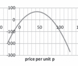
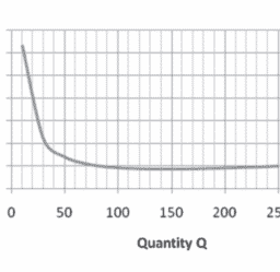
Figure 7.1 illustrates how $Z^(\theta)$, the objective function value for the optimal solution (given $\theta$ ), changes as $\theta$ increases. In fact, $Z^(\theta)$ always has this piecewise linear and convex ${ }^1$ form (see Prob. 7.2-7). The corresponding optimal solution changes (as $\theta$ increases) just at the values of $\theta$ where the slope of the $Z^(\theta)$ function changes. Thus, Fig. 7.1 depicts a problem where three different solutions are optimal for different values of $\theta$, the first for $0 \leq \theta \leq \theta_1$, the second for $\theta_1 \leq \theta \leq \theta_2$, and the third for $\theta \geq \theta_2$. Because the value of each $x_j$ remains the same within each of these intervals for $\theta$, the value of $Z^(\theta)$ varies with $\theta$ only because the coefficients of the $x_j$ are changing as a linear function of $\theta$. The solution procedure is based directly upon the sensitivity analysis procedure for investigating changes in the $c_j$ parameters (Cases $2 a$ and 3 , Sec. 6.7). As described in the last subsection of Sec. 6.7, the only basic difference with parametric linear programming is that the changes now are expressed in terms of $\theta$ rather than as specific numbers.
数学代写|运筹学代写Operations Research代考|Systematic Changes in the $b_i$ Parameters
For the case where the $b_i$ parameters change systematically, the one modification made in the original linear programming model is that $b_i$ is replaced by $b_i+\alpha_i \theta$, for $i=1$, $2, \ldots, m$, where the $\alpha_i$ are given input constants. Thus, the problem becomes
$$
\text { Maximize } Z(\theta)=\sum_{j=1}^n c_j x_j
$$
subject to
$$
\sum_{j=1}^n a_{i j} x_j \leq b_i+\alpha_i \theta \quad \text { for } i=1,2, \ldots, m
$$
and
$$
x_j \geq 0 \quad \text { for } j=1,2, \ldots, n .
$$
The goal is to identify the optimal solution as a function of $\theta$.
With this formulation, the corresponding objective function value $Z^(\theta)$ always has the piecewise linear and concave $e^1$ form shown in Fig. 7.2. (See Prob. 7.2-8.) The set of basic variables in the optimal solution still changes (as $\theta$ increases) only where the slope of $Z^(\theta)$ changes. However, in contrast to the preceding case, the values of these variables now change as a (linear) function of $\theta$ between the slope changes. The reason is that increasing $\theta$ changes the right-hand sides in the initial set of equations, which then causes changes in the right-hand sides in the final set of equations, i.e., in the values of the final set of basic variables. Figure 7.2 depicts a problem with three sets of basic variables that are optimal for different values of $\theta$, the first for $0 \leq \theta \leq \theta_1$, the second for $\theta_1 \leq \theta \leq \theta_2$, and the third for $\theta \geq \theta_2$. Within each of these intervals of $\theta$, the value of $Z *(\theta)$ varies with $\theta$ despite the fixed coefficients $c_j$ because the $x_j$ values are changing.
The following solution procedure summary is very similar to that just presented for systematic changes in the $c_j$ parameters. The reason is that changing the $b_i$ values is equivalent to changing the coefficients in the objective function of the dual model. Therefore, the procedure for the primal problem is exactly complementary to applying simultaneously the procedure for systematic changes in the $c_j$ parameters to the dual problem. Consequently, the dual simplex method (see Sec. 7.1) now would be used to obtain each new optimal solution, and the applicable sensitivity analysis case (see Sec. 6.7) now is Case 1 , but these differences are the only major differences.
运筹学代写
数学代写|运筹学代写Operations Research代考|Systematic Changes in the $c_j$ Parameters
对于$c_j$参数发生变化的情况,一般线性规划模型的目标函数
$$
Z=\sum_{j=1}^n c_j x_j
$$
被
$$
Z(\theta)=\sum_{j=1}^n\left(c_{j+} \alpha_j \theta\right) x_j,
$$
其中$\alpha_j$给出了代表系数变化的相对速率的输入常数。因此,从零开始逐渐增加$\theta$会以这些相对速率改变系数。
分配给$\alpha_j$的值可能代表$c_j$的有趣的同时变化,用于增加这些变化幅度的影响的系统灵敏度分析。它们也可能基于系数(例如,单位利润)如何与$\theta$测量的某些因素一起变化。这个因素可能是无法控制的,例如,经济状况。但是,它也可能在决策者的控制之下,例如,从某些活动转移到其他活动的人员和设备的数量。
对于任意给定的$\theta$值,可以用单纯形法得到相应线性规划问题的最优解。对于原来的问题,这个解决方案可能已经得到了$\theta=0$。然而,目标是找到修正线性规划问题的最优解[在原始约束下最大化$Z(\theta)$]作为$\theta$的函数。因此,在求解过程中,您需要能够确定当$\theta$从零增加到任何指定的正数时,最优解何时以及如何变化(如果确实如此)。
图7.1说明了最优解(给定$\theta$)的目标函数值$Z^(\theta)$如何随着$\theta$的增加而变化。事实上,$Z^(\theta)$总是有这种分段线性和凸${ }^1$形式(见问题7.2-7)。对应的最优解在$Z^(\theta)$函数斜率变化的$\theta$处发生变化(随着$\theta$的增加)。因此,图7.1描述了一个问题,其中三个不同的解对于不同的$\theta$值是最优的,第一个解对于$0 \leq \theta \leq \theta_1$,第二个解对于$\theta_1 \leq \theta \leq \theta_2$,第三个解对于$\theta \geq \theta_2$。因为每个$x_j$的值在$\theta$的每个区间内保持不变,所以$Z^(\theta)$的值随$\theta$变化只是因为$x_j$的系数作为$\theta$的线性函数而变化。解决程序直接基于调查$c_j$参数变化的敏感性分析程序(案例$2 a$和3,第6.7节)。正如第6.7节最后一节所描述的,与参数线性规划的唯一基本区别是,现在的变化是用$\theta$而不是具体的数字来表示的。
数学代写|运筹学代写Operations Research代考|Systematic Changes in the $b_i$ Parameters
对于$b_i$参数系统变化的情况,在原始线性规划模型中所做的一个修改是将$b_i$替换为$b_i+\alpha_i \theta$,对于$i=1$, $2, \ldots, m$,其中$\alpha_i$是给定的输入常量。因此,问题就变成了
$$
\text { Maximize } Z(\theta)=\sum_{j=1}^n c_j x_j
$$
以
$$
\sum_{j=1}^n a_{i j} x_j \leq b_i+\alpha_i \theta \quad \text { for } i=1,2, \ldots, m
$$
和
$$
x_j \geq 0 \quad \text { for } j=1,2, \ldots, n .
$$
目标是确定作为$\theta$函数的最优解决方案。
在此公式下,对应的目标函数值$Z^(\theta)$始终为图7.2所示的分段线性凹$e^1$形式。(见箴言7.2-8)最优解中的基本变量集只在$Z^(\theta)$的斜率变化时才会发生变化(随着$\theta$的增加)。然而,与前面的情况相反,这些变量的值现在在斜率变化之间作为$\theta$的(线性)函数变化。原因是增加$\theta$会改变初始方程的右侧,从而导致最终方程的右侧发生变化,即最终基本变量集的值发生变化。图7.2描述了一个具有三组基本变量的问题,它们对于不同的$\theta$值是最优的,第一组用于$0 \leq \theta \leq \theta_1$,第二组用于$\theta_1 \leq \theta \leq \theta_2$,第三组用于$\theta \geq \theta_2$。在$\theta$的每个区间内,尽管系数是固定的$c_j$,但$Z *(\theta)$的值随着$\theta$而变化,因为$x_j$的值在变化。
下面的解决方案过程总结与刚才介绍的$c_j$参数的系统更改非常相似。其原因是改变$b_i$值相当于改变对偶模型目标函数中的系数。因此,原始问题的处理过程与同时将$c_j$参数系统变化的处理过程应用于对偶问题是完全互补的。因此,现在将使用对偶单纯形方法(参见7.1节)来获得每个新的最优解,现在适用的敏感性分析案例(参见6.7节)是案例1,但这些差异是唯一的主要差异。

数学代写|运筹学代写Operations Research代考 请认准UprivateTA™. UprivateTA™为您的留学生涯保驾护航。
微观经济学代写
微观经济学是主流经济学的一个分支,研究个人和企业在做出有关稀缺资源分配的决策时的行为以及这些个人和企业之间的相互作用。my-assignmentexpert™ 为您的留学生涯保驾护航 在数学Mathematics作业代写方面已经树立了自己的口碑, 保证靠谱, 高质且原创的数学Mathematics代写服务。我们的专家在图论代写Graph Theory代写方面经验极为丰富,各种图论代写Graph Theory相关的作业也就用不着 说。
线性代数代写
线性代数是数学的一个分支,涉及线性方程,如:线性图,如:以及它们在向量空间和通过矩阵的表示。线性代数是几乎所有数学领域的核心。
博弈论代写
现代博弈论始于约翰-冯-诺伊曼(John von Neumann)提出的两人零和博弈中的混合策略均衡的观点及其证明。冯-诺依曼的原始证明使用了关于连续映射到紧凑凸集的布劳威尔定点定理,这成为博弈论和数学经济学的标准方法。在他的论文之后,1944年,他与奥斯卡-莫根斯特恩(Oskar Morgenstern)共同撰写了《游戏和经济行为理论》一书,该书考虑了几个参与者的合作游戏。这本书的第二版提供了预期效用的公理理论,使数理统计学家和经济学家能够处理不确定性下的决策。
微积分代写
微积分,最初被称为无穷小微积分或 “无穷小的微积分”,是对连续变化的数学研究,就像几何学是对形状的研究,而代数是对算术运算的概括研究一样。
它有两个主要分支,微分和积分;微分涉及瞬时变化率和曲线的斜率,而积分涉及数量的累积,以及曲线下或曲线之间的面积。这两个分支通过微积分的基本定理相互联系,它们利用了无限序列和无限级数收敛到一个明确定义的极限的基本概念 。
计量经济学代写
什么是计量经济学?
计量经济学是统计学和数学模型的定量应用,使用数据来发展理论或测试经济学中的现有假设,并根据历史数据预测未来趋势。它对现实世界的数据进行统计试验,然后将结果与被测试的理论进行比较和对比。
根据你是对测试现有理论感兴趣,还是对利用现有数据在这些观察的基础上提出新的假设感兴趣,计量经济学可以细分为两大类:理论和应用。那些经常从事这种实践的人通常被称为计量经济学家。
Matlab代写
MATLAB 是一种用于技术计算的高性能语言。它将计算、可视化和编程集成在一个易于使用的环境中,其中问题和解决方案以熟悉的数学符号表示。典型用途包括:数学和计算算法开发建模、仿真和原型制作数据分析、探索和可视化科学和工程图形应用程序开发,包括图形用户界面构建MATLAB 是一个交互式系统,其基本数据元素是一个不需要维度的数组。这使您可以解决许多技术计算问题,尤其是那些具有矩阵和向量公式的问题,而只需用 C 或 Fortran 等标量非交互式语言编写程序所需的时间的一小部分。MATLAB 名称代表矩阵实验室。MATLAB 最初的编写目的是提供对由 LINPACK 和 EISPACK 项目开发的矩阵软件的轻松访问,这两个项目共同代表了矩阵计算软件的最新技术。MATLAB 经过多年的发展,得到了许多用户的投入。在大学环境中,它是数学、工程和科学入门和高级课程的标准教学工具。在工业领域,MATLAB 是高效研究、开发和分析的首选工具。MATLAB 具有一系列称为工具箱的特定于应用程序的解决方案。对于大多数 MATLAB 用户来说非常重要,工具箱允许您学习和应用专业技术。工具箱是 MATLAB 函数(M 文件)的综合集合,可扩展 MATLAB 环境以解决特定类别的问题。可用工具箱的领域包括信号处理、控制系统、神经网络、模糊逻辑、小波、仿真等。