如果你也在 怎样代写运筹学Operations Research 这个学科遇到相关的难题,请随时右上角联系我们的24/7代写客服。运筹学Operations Research(英式英语:operational research),通常简称为OR,是一门研究开发和应用先进的分析方法来改善决策的学科。它有时被认为是数学科学的一个子领域。管理科学一词有时被用作同义词。
运筹学Operations Research采用了其他数学科学的技术,如建模、统计和优化,为复杂的决策问题找到最佳或接近最佳的解决方案。由于强调实际应用,运筹学与许多其他学科有重叠之处,特别是工业工程。运筹学通常关注的是确定一些现实世界目标的极端值:最大(利润、绩效或收益)或最小(损失、风险或成本)。运筹学起源于二战前的军事工作,它的技术已经发展到涉及各种行业的问题。
运筹学Operations Research代写,免费提交作业要求, 满意后付款,成绩80\%以下全额退款,安全省心无顾虑。专业硕 博写手团队,所有订单可靠准时,保证 100% 原创。 最高质量的运筹学Operations Research作业代写,服务覆盖北美、欧洲、澳洲等 国家。 在代写价格方面,考虑到同学们的经济条件,在保障代写质量的前提下,我们为客户提供最合理的价格。 由于作业种类很多,同时其中的大部分作业在字数上都没有具体要求,因此运筹学Operations Research作业代写的价格不固定。通常在专家查看完作业要求之后会给出报价。作业难度和截止日期对价格也有很大的影响。
同学们在留学期间,都对各式各样的作业考试很是头疼,如果你无从下手,不如考虑my-assignmentexpert™!
my-assignmentexpert™提供最专业的一站式服务:Essay代写,Dissertation代写,Assignment代写,Paper代写,Proposal代写,Proposal代写,Literature Review代写,Online Course,Exam代考等等。my-assignmentexpert™专注为留学生提供Essay代写服务,拥有各个专业的博硕教师团队帮您代写,免费修改及辅导,保证成果完成的效率和质量。同时有多家检测平台帐号,包括Turnitin高级账户,检测论文不会留痕,写好后检测修改,放心可靠,经得起任何考验!
想知道您作业确定的价格吗? 免费下单以相关学科的专家能了解具体的要求之后在1-3个小时就提出价格。专家的 报价比上列的价格能便宜好几倍。
我们在数学Mathematics代写方面已经树立了自己的口碑, 保证靠谱, 高质且原创的数学Mathematics代写服务。我们的专家在运筹学Operations Research代写方面经验极为丰富,各种运筹学Operations Research相关的作业也就用不着 说。
数学代写|运筹学代写Operations Research代考|A STREAMLINED SIMPLEX METHOD FOR THE TRANSPORTATION PROBLEM
Because the transportation problem is just a special type of linear programming problem, it can be solved by applying the simplex method as described in Chap. 4. However, you will see in this section that some tremendous computational shortcuts can be taken in this method by exploiting the special structure shown in Table 8.6. We shall refer to this streamlined procedure as the transportation simplex method.
As you read on, note particularly how the special structure is exploited to achieve great computational savings. This will illustrate an important OR technique-streamlining an algorithm to exploit the special structure in the problem at hand.
Setting Up the Transportation Simplex Method
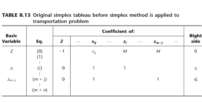
To highlight the streamlining achieved by the transportation simplex method, let us first review how the general (unstreamlined) simplex method would set up a transportation problem in tabular form. After constructing the table of constraint coefficients (see Table 8.6), converting the objective function to maximization form, and using the Big $M$ method to introduce artificial variables $z_1, z_2, \ldots, z_{m+n}$ into the $m+n$ respective equality constraints (see Sec. 4.6), typical columns of the simplex tableau would have the form shown in Table 8.13 , where all entries not shown in these columns are zeros. [The one remaining adjustment to be made before the first iteration of the simplex method is to algebraically eliminate the nonzero coefficients of the initial (artificial) basic variables in row 0.]
After any subsequent iteration, row 0 then would have the form shown in Table 8.14. Because of the pattern of $0 \mathrm{~s}$ and $1 \mathrm{~s}$ for the coefficients in Table 8.13, by the fundamental insight presented in Sec. 5.3, $u_i$ and $v_j$ would have the following interpretation:
$u_i=$ multiple of original row $i$ that has been subtracted (directly or indirectly) from original row 0 by the simplex method during all iterations leading to the current simplex tableau.
$v_j=$ multiple of original row $m+j$ that has been subtracted (directly or indirectly) from original row 0 by the simplex method during all iterations leading to the current simplex tableau.
Using the duality theory introduced in Chap. 6, another property of the $u_i$ and $v_j$ is that they are the dual variables. ${ }^1$ If $x_{i j}$ is a nonbasic variable, $c_{i j}-u_i-v_j$ is interpreted as the rate at which $Z$ will change as $x_{i j}$ is increased.
To lay the groundwork for simplifying this setup, recall what information is needed by the simplex method. In the initialization, an initial BF solution must be obtained, which is done artificially by introducing artificial variables as the initial basic variables and setting them equal to $s_i$ and $d_j$. The optimality test and step 1 of an iteration (selecting an entering basic variable) require knowing the current row 0 , which is obtained by subtracting a certain multiple of another row from the preceding row 0. Step 2 (determining the leaving basic variable) must identify the basic variable that reaches zero first as the entering basic variable is increased, which is done by comparing the current coefficients of the entering basic variable and the corresponding right side. Step 3 must determine the new BF solution, which is found by subtracting certain multiples of one row from the other rows in the current simplex tableau.
数学代写|运筹学代写Operations Research代考|Initialization
Recall that the objective of the initialization is to obtain an initial BF solution. Because all the functional constraints in the transportation problem are equality constraints, the simplex method would obtain this solution by introducing artificial variables and using them as the initial basic variables, as described in Sec. 4.6. The resulting basic solution actually is feasible only for a revised version of the problem, so a number of iterations are needed to drive these artificial variables to zero in order to reach the real BF solutions. The transportation simplex method bypasses all this by instead using a simpler procedure to directly construct a real BF solution on a transportation simplex tableau.
Before outlining this procedure, we need to point out that the number of basic variables in any basic solution of a transportation problem is one fewer than you might expect. Ordinarily, there is one basic variable for each functional constraint in a linear programming problem. For transportation problems with $m$ sources and $n$ destinations, the number of functional constraints is $m+n$. However,
Number of basic variables $=m+n-1$.
The reason is that the functional constraints are equality constraints, and this set of $m+n$ equations has one extra (or redundant) equation that can be deleted without changing the feasible region; i.e., any one of the constraints is automatically satisfied whenever the other $m+n-1$ constraints are satisfied. (This fact can be verified by showing that any supply constraint exactly equals the sum of the demand constraints minus the sum of the other supply constraints, and that any demand equation also can be reproduced by summing the supply equations and subtracting the other demand equations. See Prob.
8.2-21.) Therefore, any $B F$ solution appears on a transportation simplex tableau with exactly $m+n-1$ circled nonnegative allocations, where the sum of the allocations for each row or column equals its supply or demand. ${ }^1$
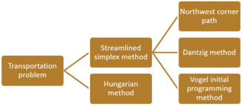
The procedure for constructing an initial BF solution selects the $m+n-1$ basic variables one at a time. After each selection, a value that will satisfy one additional constraint (thereby eliminating that constraint’s row or column from further consideration for providing allocations) is assigned to that variable. Thus, after $m+n-1$ selections, an entire basic solution has been constructed in such a way as to satisfy all the constraints. A number of different criteria have been proposed for selecting the basic variables. We present and illustrate three of these criteria here, after outlining the general procedure.
运筹学代写
数学代写|运筹学代写Operations Research代考|A STREAMLINED SIMPLEX METHOD FOR THE TRANSPORTATION PROBLEM
由于运输问题只是一种特殊类型的线性规划问题,因此可以采用第四章中描述的单纯形方法来求解。然而,在本节中您将看到,通过利用表8.6中所示的特殊结构,这种方法可以获得一些巨大的计算捷径。我们将把这种简化的程序称为运输单纯形法。
当您继续阅读时,请特别注意如何利用这种特殊结构来实现巨大的计算节省。这将说明一种重要的OR技术-简化算法以利用手头问题中的特殊结构。
建立运输单纯形法
为了强调运输单纯形方法所实现的流线型,让我们首先回顾一下一般(非流线型)单纯形方法如何以表格形式建立运输问题。在构造约束系数表(见表8.6),将目标函数转换为最大化形式,并使用Big $M$方法将人工变量$z_1, z_2, \ldots, z_{M +n}$引入$M +n$各自的等式约束(见第4.6节)之后,单纯形表的典型列将具有表8.13所示的形式,其中未在这些列中显示的所有项都为零。[在单纯形法第一次迭代之前需要做的一个调整是用代数方法消除第0行初始(人工)基本变量的非零系数。]
在任何后续迭代之后,第0行将具有表8.14所示的形式。由于表8.13中的系数为$0 \mathrm{~s}$和$1 \mathrm{~s}$的模式,根据5.3节介绍的基本见解,$u_i$和$v_j$将具有以下解释:
$u_i=$原始行$i$的倍数,在导致当前单纯形表的所有迭代中,通过单纯形方法从原始行0中(直接或间接)减去。
$v_j=$原始行$m+j$的倍数,在导致当前单纯形表的所有迭代中,单纯形方法已经从原始行0中(直接或间接)减去了j$。
利用第六章介绍的对偶理论,$u_i$和$v_j$的另一个性质是它们是对偶变量。${}^1$如果$x_{i j}$是一个非基本变量,$c_{i j}-u_i-v_j$被解释为$Z$随着$x_{i j}$的增加而变化的速率。
为了为简化此设置奠定基础,请回忆一下simplex方法需要哪些信息。在初始化中,必须获得初始BF解,这是通过引入人工变量作为初始基本变量并设置它们等于$s_i$和$d_j$来人为地完成的。迭代的最优性测试和第1步(选择一个进入的基本变量)需要知道当前的行0,这是通过从前面的行0减去另一行的某个倍数得到的。第二步(确定离开基本变量)必须通过比较进入基本变量与对应右侧的当前系数,确定随着进入基本变量的增加,首先达到零的基本变量。步骤3必须确定新的BF解,这是通过从当前单纯形表中的其他行中减去一行的某些倍数来找到的。
数学代写|运筹学代写Operations Research代考|Initialization
回想一下,初始化的目标是获得初始BF解。由于运输问题中所有的功能约束都是等式约束,因此单纯形法通过引入人工变量并将其作为初始基本变量来获得此解,如第4.6节所述。最终的基本解决方案实际上只适用于问题的修订版本,因此需要大量的迭代来驱动这些人为变量为零,以达到真正的BF解决方案。运输单纯形法通过使用一个更简单的过程来直接在运输单纯形表上构造一个真实的BF解,从而绕过了所有这些问题。
在概述这个过程之前,我们需要指出,在运输问题的任何基本解决方案中,基本变量的数量比您可能期望的要少一个。通常,线性规划问题中的每个函数约束都有一个基本变量。对于具有$m$来源和$n$目的地的运输问题,功能约束的数量为$m+n$。然而,
基本变量的个数$=m+n-1$。
原因是函数约束是等式约束,这组$m+n$方程有一个额外的(或冗余的)方程,可以在不改变可行域的情况下删除;也就是说,当其他$m+n-1$约束得到满足时,任何一个约束都会自动得到满足。(这一事实可以通过证明任何供给约束恰好等于需求约束的总和减去其他供给约束的总和来验证,并且任何需求方程也可以通过供给方程的总和减去其他需求方程来重现。看到问题。
8.2 -21年。)因此,任何$B $ F$的解决方案都出现在运输单纯形表中,具有正好$m+n-1$圈出的非负分配,其中每行或每列的分配总和等于其供给或需求。${} ^ 1美元
构造初始BF解的过程每次选择一个$m+n-1$基本变量。在每次选择之后,将满足一个附加约束的值赋给该变量(从而在提供分配时不再进一步考虑该约束的行或列)。因此,在$m+n-1$选择之后,以满足所有约束的方式构造了一个完整的基本解。对于选择基本变量,已经提出了若干不同的标准。在概述了一般程序之后,我们在这里提出并说明其中的三个标准。

数学代写|运筹学代写Operations Research代考 请认准UprivateTA™. UprivateTA™为您的留学生涯保驾护航。
微观经济学代写
微观经济学是主流经济学的一个分支,研究个人和企业在做出有关稀缺资源分配的决策时的行为以及这些个人和企业之间的相互作用。my-assignmentexpert™ 为您的留学生涯保驾护航 在数学Mathematics作业代写方面已经树立了自己的口碑, 保证靠谱, 高质且原创的数学Mathematics代写服务。我们的专家在图论代写Graph Theory代写方面经验极为丰富,各种图论代写Graph Theory相关的作业也就用不着 说。
线性代数代写
线性代数是数学的一个分支,涉及线性方程,如:线性图,如:以及它们在向量空间和通过矩阵的表示。线性代数是几乎所有数学领域的核心。
博弈论代写
现代博弈论始于约翰-冯-诺伊曼(John von Neumann)提出的两人零和博弈中的混合策略均衡的观点及其证明。冯-诺依曼的原始证明使用了关于连续映射到紧凑凸集的布劳威尔定点定理,这成为博弈论和数学经济学的标准方法。在他的论文之后,1944年,他与奥斯卡-莫根斯特恩(Oskar Morgenstern)共同撰写了《游戏和经济行为理论》一书,该书考虑了几个参与者的合作游戏。这本书的第二版提供了预期效用的公理理论,使数理统计学家和经济学家能够处理不确定性下的决策。
微积分代写
微积分,最初被称为无穷小微积分或 “无穷小的微积分”,是对连续变化的数学研究,就像几何学是对形状的研究,而代数是对算术运算的概括研究一样。
它有两个主要分支,微分和积分;微分涉及瞬时变化率和曲线的斜率,而积分涉及数量的累积,以及曲线下或曲线之间的面积。这两个分支通过微积分的基本定理相互联系,它们利用了无限序列和无限级数收敛到一个明确定义的极限的基本概念 。
计量经济学代写
什么是计量经济学?
计量经济学是统计学和数学模型的定量应用,使用数据来发展理论或测试经济学中的现有假设,并根据历史数据预测未来趋势。它对现实世界的数据进行统计试验,然后将结果与被测试的理论进行比较和对比。
根据你是对测试现有理论感兴趣,还是对利用现有数据在这些观察的基础上提出新的假设感兴趣,计量经济学可以细分为两大类:理论和应用。那些经常从事这种实践的人通常被称为计量经济学家。
Matlab代写
MATLAB 是一种用于技术计算的高性能语言。它将计算、可视化和编程集成在一个易于使用的环境中,其中问题和解决方案以熟悉的数学符号表示。典型用途包括:数学和计算算法开发建模、仿真和原型制作数据分析、探索和可视化科学和工程图形应用程序开发,包括图形用户界面构建MATLAB 是一个交互式系统,其基本数据元素是一个不需要维度的数组。这使您可以解决许多技术计算问题,尤其是那些具有矩阵和向量公式的问题,而只需用 C 或 Fortran 等标量非交互式语言编写程序所需的时间的一小部分。MATLAB 名称代表矩阵实验室。MATLAB 最初的编写目的是提供对由 LINPACK 和 EISPACK 项目开发的矩阵软件的轻松访问,这两个项目共同代表了矩阵计算软件的最新技术。MATLAB 经过多年的发展,得到了许多用户的投入。在大学环境中,它是数学、工程和科学入门和高级课程的标准教学工具。在工业领域,MATLAB 是高效研究、开发和分析的首选工具。MATLAB 具有一系列称为工具箱的特定于应用程序的解决方案。对于大多数 MATLAB 用户来说非常重要,工具箱允许您学习和应用专业技术。工具箱是 MATLAB 函数(M 文件)的综合集合,可扩展 MATLAB 环境以解决特定类别的问题。可用工具箱的领域包括信号处理、控制系统、神经网络、模糊逻辑、小波、仿真等。