如果你也在 怎样代写广义线性模型Generalized linear model 这个学科遇到相关的难题,请随时右上角联系我们的24/7代写客服。广义线性模型Generalized linear model在统计学中,是普通线性回归的灵活概括。广义线性模型通过允许线性模型通过一个链接函数与响应变量相关,并允许每个测量值的方差大小是其预测值的函数,从而概括了线性回归。
广义线性模型Generalized linear model是由John Nelder和Robert Wedderburn提出的,作为统一其他各种统计模型的一种方式,包括线性回归、逻辑回归和泊松回归。他们提出了一种迭代加权的最小二乘法,用于模型参数的最大似然估计。最大似然估计仍然很流行,是许多统计计算软件包的默认方法。其他方法,包括贝叶斯方法和最小二乘法对方差稳定反应的拟合,已经被开发出来。
广义线性模型Generalized linear model代写,免费提交作业要求, 满意后付款,成绩80\%以下全额退款,安全省心无顾虑。专业硕 博写手团队,所有订单可靠准时,保证 100% 原创。最高质量的广义线性模型Generalized linear model作业代写,服务覆盖北美、欧洲、澳洲等 国家。 在代写价格方面,考虑到同学们的经济条件,在保障代写质量的前提下,我们为客户提供最合理的价格。 由于作业种类很多,同时其中的大部分作业在字数上都没有具体要求,因此广义线性模型Generalized linear model作业代写的价格不固定。通常在专家查看完作业要求之后会给出报价。作业难度和截止日期对价格也有很大的影响。
同学们在留学期间,都对各式各样的作业考试很是头疼,如果你无从下手,不如考虑my-assignmentexpert™!
my-assignmentexpert™提供最专业的一站式服务:Essay代写,Dissertation代写,Assignment代写,Paper代写,Proposal代写,Proposal代写,Literature Review代写,Online Course,Exam代考等等。my-assignmentexpert™专注为留学生提供Essay代写服务,拥有各个专业的博硕教师团队帮您代写,免费修改及辅导,保证成果完成的效率和质量。同时有多家检测平台帐号,包括Turnitin高级账户,检测论文不会留痕,写好后检测修改,放心可靠,经得起任何考验!
想知道您作业确定的价格吗? 免费下单以相关学科的专家能了解具体的要求之后在1-3个小时就提出价格。专家的 报价比上列的价格能便宜好几倍。
我们在统计Statistics代写方面已经树立了自己的口碑, 保证靠谱, 高质且原创的统计Statistics代写服务。我们的专家在广义线性模型Generalized linear model代写方面经验极为丰富,各种广义线性模型Generalized linear model相关的作业也就用不着说。
统计代写|广义线性模型代写Generalized linear model代考|Expected versus observed information matrix
One can adjust the IRLS estimating algorithm such that the observed information matrix is used rather than the expected matrix. One need only create
$$
W_o=W+(y-\mu)\left{\frac{v g^{\prime \prime}+v^{\prime} g^{\prime}}{v^2\left(g^{\prime}\right)^3}\right}
$$
Here $g^{\prime}=g^{\prime}(\mu)$, the derivative of the link; $g^{\prime \prime}=g^{\prime \prime}(\mu)$, the second derivative of the link; $v=v(\mu)$, the variance function; $v^2=$ variance squared; and $W$ is the standard IRLS weight function given in (3.46).
The generic form of the GLM IRLS algorithm, using the observed information matrix, is then given by
Listing 5.4: IRLS algorithm for GLM using OIM
$\mu={y+\operatorname{mean}(y)} / 2$
$\eta=g$
WHILE $(\operatorname{abs}(\Delta$ Dev $)>$ tolerance $){$
$W=1\left(v g^{\prime 2}\right)$
$z=\eta+(y-\mu) g^{\prime}-$ offset
$W_o=W+(y-\mu)\left(v g^{\prime \prime}+v^{\prime} g^{\prime}\right)\left(v^2\left(g^{\prime}\right)^3\right)$
$\boldsymbol{\beta}=\left(X^T W_0 X\right)^{-1} X^T W_0 z$
$\eta=X \boldsymbol{\beta}+$ offset
$\mu=g^{-1}$
OldDev $=$ Dev
Dev $=\sum$ (deviance function)
$\Delta$ Dev $=$ Dev – OldDev
3
$x^2=\sum(y-\mu)^2 N$
where $V^{\prime}$ is the derivative with respect to $\mu$ of the variance function.
Using this algorithm, which we will call the IRLS-OIM algorithm, estimates and standard errors will be identical to those produced using ML. The scale, estimated by the ML routine, is estimated as the deviance-based dispersion. However, unlike ML output, the IRLS-OIM algorithm fails to provide standard errors for the scale. Of course, the benefit to using IRLS-OIM is that the typical ML problems with starting values are nearly always avoided. Also, ML routines usually take a bit longer to converge than does a straightforward IRLS-OIM algorithm.
统计代写|广义线性模型代写Generalized linear model代考|Other Gaussian links
The standard or normal linear model, obs regression, uses the identity link, which is the canonical form of the distribution. It is robust to most minor violations of Gaussian distributional assumptions but is used in more data modeling situations than is appropriate. In fact, it was used to model binary, proportional, and discrete count data. Appropriate software was unavailable, and there was not widespread understanding of the statistical problems inherent in using ols regression for data modeling.
There is no theoretical reason why researchers using the Gaussian family for a model should be limited to using only the identity or log links. The reciprocal link, $1 / \mu$, has been used to model data with a rate response. It also may be desirable to use the power links with the Gaussian model. In doing so, we approximate the Box-Cox ML algorithm, which is used as a normality transform. Some software packages do not have Box-Cox capabilities; therefore, using power links with the Gaussian family may assist in achieving the same purpose.
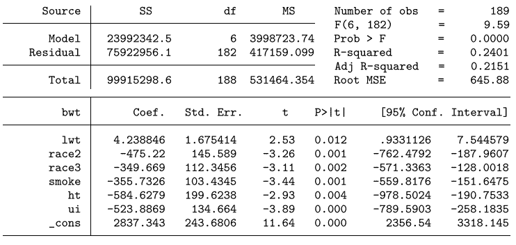
We provide a simple example showing the relationship of oLs regression output to that of GLM. The example we use comes from a widely used study on prediction of low-birth-weight babies (Hosmer, Lemeshow, and Sturdivant 2013). The response variable, bwt, is the birth weight of the baby. The predictors are lwt, the weight of the mother; race, where a value of 1 indicates white, 2 indicates black, and 3 indicates other; a binary variable, smoke, which indicates whether the mother has a history of smoking; another binary variable ht, which indicates whether the mother has a history of hypertension; and a final binary variable ui, which indicates whether the mother has a history of uterine irritability. We generated indicator variables for use in model specification race2 indicating black and race3 indicating other. The standard Stata regression output is given by
. use http://www.stata-press.com/data/hh4/lbw
(Hosmer \& Lemeshow data)
regress bwt lwt race 2 race3 smoke ht ui

广义线性模型代写
统计代写|广义线性模型代写Generalized linear model代考|Expected versus observed information matrix
可以调整IRLS估计算法,以便使用观察到的信息矩阵而不是期望的矩阵。只需要创建
$$
W_o=W+(y-\mu)\left{\frac{v g^{\prime \prime}+v^{\prime} g^{\prime}}{v^2\left(g^{\prime}\right)^3}\right}
$$
这里$g^{\prime}=g^{\prime}(\mu)$,链接的导数;$g^{\prime \prime}=g^{\prime \prime}(\mu)$,连杆的二阶导数;$v=v(\mu)$,方差函数;$v^2=$方差平方;$W$为(3.46)中给出的标准IRLS权重函数。
利用观测到的信息矩阵,给出了GLM IRLS算法的一般形式
清单5.4:使用OIM的GLM的IRLS算法
$\mu={y+\operatorname{mean}(y)} / 2$
$\eta=g$
虽然$(\operatorname{abs}(\Delta$开发$)>$宽容$){$
$W=1\left(v g^{\prime 2}\right)$
$z=\eta+(y-\mu) g^{\prime}-$偏移
$W_o=W+(y-\mu)\left(v g^{\prime \prime}+v^{\prime} g^{\prime}\right)\left(v^2\left(g^{\prime}\right)^3\right)$
$\boldsymbol{\beta}=\left(X^T W_0 X\right)^{-1} X^T W_0 z$
$\eta=X \boldsymbol{\beta}+$偏移
$\mu=g^{-1}$
OldDev $=$ Dev
Dev $=\sum$(偏差功能)
$\Delta$ Dev $=$ Dev – OldDev
3.
$x^2=\sum(y-\mu)^2 N$
其中$V^{\prime}$是方差函数对$\mu$的导数。
使用这种算法,我们将其称为IRLS-OIM算法,估计和标准误差将与使用ML产生的估计和标准误差相同。由ML例程估计的尺度被估计为基于偏差的离散度。然而,与ML输出不同,IRLS-OIM算法无法提供尺度的标准误差。当然,使用IRLS-OIM的好处是,几乎总是可以避免带有初始值的典型ML问题。此外,ML例程通常比直接的IRLS-OIM算法需要更长的时间来收敛。
统计代写|广义线性模型代写Generalized linear model代考|Other Gaussian links
标准或正态线性模型,即回归,使用恒等链,这是分布的规范形式。它对高斯分布假设的大多数轻微违反具有鲁棒性,但在更多的数据建模情况下使用比合适的。事实上,它被用来模拟二进制、比例和离散计数数据。没有适当的软件,而且对使用ols回归进行数据建模所固有的统计问题也没有广泛的了解。
没有理论上的理由说明为什么研究人员使用高斯族的模型应该仅限于使用恒等或日志链接。反向链接$1 / \mu$已被用于对具有速率响应的数据进行建模。在高斯模型中使用功率链路也是可取的。在这样做时,我们近似Box-Cox ML算法,它被用作正态变换。有些软件包不具备Box-Cox功能;因此,使用高斯族的功率链路可能有助于实现相同的目的。
我们提供了一个简单的例子来展示oLs回归输出与GLM的关系。我们使用的例子来自一项广泛使用的关于低出生体重婴儿预测的研究(Hosmer, Lemeshow, and Sturdivant 2013)。响应变量bwt是婴儿的出生体重。预测因子是lwt,母亲的体重;种族,1表示白色,2表示黑色,3表示其他;一个二元变量,吸烟,这表明母亲是否有吸烟史;另一个二元变量ht,表明母亲是否有高血压病史;最后一个二元变量ui,表示母亲是否有子宫易怒史。我们生成了用于模型规范的指示变量race2表示黑色,race3表示其他。标准Stata回归输出由
. 使用http://www.stata-press.com/data/hh4/lbw
(Hosmer & Lemeshow数据)
回归BWT LWT race 2 race3 smoke ht UI

统计代写|广义线性模型代写Generalized linear model代考 请认准UprivateTA™. UprivateTA™为您的留学生涯保驾护航。