如果你也在 怎样代写广义线性模型Generalized linear model 这个学科遇到相关的难题,请随时右上角联系我们的24/7代写客服。广义线性模型Generalized linear model通过允许响应变量具有任意分布(而不是简单的正态分布),以及响应变量的任意函数(链接函数)随预测器线性变化(而不是假设响应本身必须线性变化),涵盖了所有这些情况。例如,上面预测海滩出席人数的情况通常会用泊松分布和日志链接来建模,而预测海滩出席率的情况通常会用伯努利分布(或二项分布,取决于问题的确切表达方式)和对数-几率(或logit)链接函数来建模。
广义线性模型Generalized linear model普通线性回归将给定未知量(响应变量,随机变量)的期望值预测为一组观测值(预测因子)的线性组合。这意味着预测器的恒定变化会导致响应变量的恒定变化(即线性响应模型)。当响应变量可以在任意一个方向上以良好的近似值无限变化时,或者更一般地适用于与预测变量(例如人类身高)的变化相比仅变化相对较小的任何数量时,这是适当的。
广义线性模型Generalized linear model代写,免费提交作业要求, 满意后付款,成绩80\%以下全额退款,安全省心无顾虑。专业硕 博写手团队,所有订单可靠准时,保证 100% 原创。最高质量的广义线性模型Generalized linear model作业代写,服务覆盖北美、欧洲、澳洲等 国家。 在代写价格方面,考虑到同学们的经济条件,在保障代写质量的前提下,我们为客户提供最合理的价格。 由于作业种类很多,同时其中的大部分作业在字数上都没有具体要求,因此广义线性模型Generalized linear model作业代写的价格不固定。通常在专家查看完作业要求之后会给出报价。作业难度和截止日期对价格也有很大的影响。
同学们在留学期间,都对各式各样的作业考试很是头疼,如果你无从下手,不如考虑my-assignmentexpert™!
my-assignmentexpert™提供最专业的一站式服务:Essay代写,Dissertation代写,Assignment代写,Paper代写,Proposal代写,Proposal代写,Literature Review代写,Online Course,Exam代考等等。my-assignmentexpert™专注为留学生提供Essay代写服务,拥有各个专业的博硕教师团队帮您代写,免费修改及辅导,保证成果完成的效率和质量。同时有多家检测平台帐号,包括Turnitin高级账户,检测论文不会留痕,写好后检测修改,放心可靠,经得起任何考验!
想知道您作业确定的价格吗? 免费下单以相关学科的专家能了解具体的要求之后在1-3个小时就提出价格。专家的 报价比上列的价格能便宜好几倍。
我们在统计Statistics代写方面已经树立了自己的口碑, 保证靠谱, 高质且原创的统计Statistics代写服务。我们的专家在广义线性模型Generalized linear model代写方面经验极为丰富,各种广义线性模型Generalized linear model相关的作业也就用不着说。
统计代写|广义线性模型代写Generalized linear model代考|Shape of the distribution
The inverse Gaussian probability density function is typically defined as
$$
f(y ; \mu, \phi)=\left(\frac{\phi}{2 \pi y^3}\right)^{1 / 2} \exp \left{\frac{-\phi(y-\mu)^2}{2 \mu^2 y}\right}
$$
Although analysts rarely use this density function when modeling data, there are times when it fits the data better than other continuous models. It is especially well suited to fit positive continuous data that have a concentration of lowvalued data with a long right skew. This feature also becomes useful when mixed with the Poisson distribution to create the Poisson inverse Gaussian mixture model discussed later; see section $14.11$.
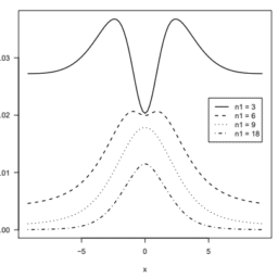
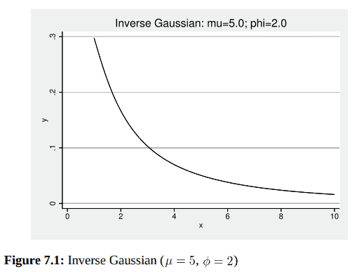
To illustrate the shape of unadjusted inverse Gaussian density functions, we create a simple set of Stata commands to generate values of the probability density function for specified mean and scale parameters. Graphs of probability density functions for various parameter values demonstrate the flexibility.
We begin with a simple function for which $\mu=5$ and $\phi=2$ shown in figure 7.1 .
$$
\begin{aligned}
& \text { twoway function } y=\exp \left((-2.0 *(x-5.0) \sim 2) /\left(2 * 5.0^{-} 2 * \mathrm{x}\right)\right) * \operatorname{sqrt}(2.0 /(2 * \text { pi*x-3)), } \
& >\text { range(1 10) title(“Inverse Gaussian: mu=5.0; phi=2.0”) }
\end{aligned}
$$
统计代写|广义线性模型代写Generalized linear model代考|The inverse Gaussian algorithm
Inserting the appropriate inverse Gaussian formulas into the standard GLM algorithm and excluding prior weights and subscripts, we have
Listing 7.1: IRLS algorithm for inverse Gaussian models
$$
\begin{aligned}
& \mu={y-\operatorname{mean}(y)} / 2 \
& \eta=1 / \mu^2 \
& \text { WHILE }(\operatorname{abs}(\Delta \mathrm{Dev})>\text { tolerance }){ \
& W=\mu^3 \
& z=\eta+(y-\mu) y \mu^3 \
& \beta=\left(X^{\mathrm{T}} W X\right)^{-1} X^{\mathrm{T}} W z \
& \eta=X \beta \
& \mu=1 / \sqrt{\eta} \
& \text { OldDev }=\text { Dev } \
& \text { Dev }=\sum(y-\mu)^2 /\left(y \mu^2\right) \
& \Delta \text { Dev }=\text { Dev }- \text { OldDev } \
& 3 \
& \chi^2=\sigma \sum(y-\mu)^2 / \mu^3 \
&
\end{aligned}
$$
We have mentioned before that the IRLS algorithm may be amended such that the log-likelihood function is used as the basis of iteration rather than the deviance. However, when this is done, the log-likelihood function itself is usually amended. The normalization term is dropped such that terms with no instance of the mean parameter, $\mu$, are excluded. Of course, prior weights are kept. For the inverse Gaussian, the amended log-likelihood function is usually given as
$$
\mathcal{L}\left(\mu, \sigma^2 ; y\right)=\sum_{i=1}^n \frac{1}{\sigma^2}\left(-\frac{y_i}{2 \mu_i^2}+\frac{1}{\mu_i}\right)
$$

广义线性模型代写
统计代写|广义线性模型代写Generalized linear model代考|Shape of the distribution
逆高斯概率密度函数通常定义为
$$
f(y ; \mu, \phi)=\left(\frac{\phi}{2 \pi y^3}\right)^{1 / 2} \exp \left{\frac{-\phi(y-\mu)^2}{2 \mu^2 y}\right}
$$
尽管分析师在建模数据时很少使用此密度函数,但有时它比其他连续模型更适合数据。它特别适合于拟合具有长右偏的低值数据集中的正连续数据。当与泊松分布混合以创建泊松逆高斯混合模型时,该特征也变得有用;参见$14.11$部分。
为了说明未调整的逆高斯密度函数的形状,我们创建了一组简单的Stata命令来为指定的平均值和尺度参数生成概率密度函数的值。各种参数值的概率密度函数图展示了这种灵活性。
我们从一个简单的函数开始,$\mu=5$和$\phi=2$如图7.1所示。
$$
\begin{aligned}
& \text { twoway function } y=\exp \left((-2.0 *(x-5.0) \sim 2) /\left(2 * 5.0^{-} 2 * \mathrm{x}\right)\right) * \operatorname{sqrt}(2.0 /(2 * \text { pi*x-3)), } \
& >\text { range(1 10) title(“Inverse Gaussian: mu=5.0; phi=2.0”) }
\end{aligned}
$$
统计代写|广义线性模型代写Generalized linear model代考|The inverse Gaussian algorithm
在标准的GLM算法中插入适当的逆高斯公式,并排除先前的权重和下标,我们有
清单7.1:逆高斯模型的IRLS算法
$$
\begin{aligned}
& \mu={y-\operatorname{mean}(y)} / 2 \
& \eta=1 / \mu^2 \
& \text { WHILE }(\operatorname{abs}(\Delta \mathrm{Dev})>\text { tolerance }){ \
& W=\mu^3 \
& z=\eta+(y-\mu) y \mu^3 \
& \beta=\left(X^{\mathrm{T}} W X\right)^{-1} X^{\mathrm{T}} W z \
& \eta=X \beta \
& \mu=1 / \sqrt{\eta} \
& \text { OldDev }=\text { Dev } \
& \text { Dev }=\sum(y-\mu)^2 /\left(y \mu^2\right) \
& \Delta \text { Dev }=\text { Dev }- \text { OldDev } \
& 3 \
& \chi^2=\sigma \sum(y-\mu)^2 / \mu^3 \
&
\end{aligned}
$$
我们之前提到过,IRLS算法可以进行修改,使对数似然函数作为迭代的基础,而不是偏差。然而,当这样做时,对数似然函数本身通常被修正。删除归一化项,以便排除没有平均参数$\mu$实例的项。当然,保留了先前的权重。对于逆高斯函数,修正后的对数似然函数通常表示为
$$
\mathcal{L}\left(\mu, \sigma^2 ; y\right)=\sum_{i=1}^n \frac{1}{\sigma^2}\left(-\frac{y_i}{2 \mu_i^2}+\frac{1}{\mu_i}\right)
$$

统计代写|广义线性模型代写Generalized linear model代考 请认准UprivateTA™. UprivateTA™为您的留学生涯保驾护航。