如果你也在 怎样代写数学分析Mathematical Analysis 这个学科遇到相关的难题,请随时右上角联系我们的24/7代写客服。数学分析Mathematical Analysis是纯数学和应用数学许多研究领域的共同基础。它也是一个重要而强大的工具,用于许多其他科学领域,包括物理,化学,生物,工程,金融,经济学,仅举几例。
数学分析Mathematical Analysis应该为最好的正则函数(即在复变量/分析中处理的解析函数)和最差的正则函数(即在实际分析中处理的可测函数)之间的函数提供一种理论。
数学分析Mathematical Analysis作业代写,免费提交作业要求, 满意后付款,成绩80\%以下全额退款,安全省心无顾虑。专业硕 博写手团队,所有订单可靠准时,保证 100% 原创, 最高质量的数学分析Mathematical Analysis作业代写,服务覆盖北美、欧洲、澳洲等 国家。 在代写价格方面,考虑到同学们的经济条件,在保障代写质量的前提下,我们为客户提供最合理的价格。 由于作业种类很多,同时其中的大部分作业在字数上都没有具体要求,因此数学分析Mathematical Analysis作业代写的价格不固定。通常在学专家查看完作业要求之后会给出报价。作业难度和截止日期对价格也有很大的影响。
同学们在留学期间,都对各式各样的作业考试很是头疼,如果你无从下手,不如考虑my-assignmentexpert™!
my-assignmentexpert™提供最专业的一站式服务:Essay代写,Dissertation代写,Assignment代写,Paper代写,Proposal代写,Proposal代写,Literature Review代写,Online Course,Exam代考等等。my-assignmentexpert™专注为留学生提供Essay代写服务,拥有各个专业的博硕教师团队帮您代写,免费修改及辅导,保证成果完成的效率和质量。同时有多家检测平台帐号,包括Turnitin高级账户,检测论文不会留痕,写好后检测修改,放心可靠,经得起任何考验!
想知道您作业确定的价格吗? 免费下单以相关学科的专家能了解具体的要求之后在1-3个小时就提出价格。专家的 报价比上列的价格能便宜好几倍。
我们在数学Mathematics代写方面已经树立了自己的口碑, 保证靠谱, 高质且原创的数学Mathematics代写服务。我们的专家在数学分析Mathematical Analysis代写方面经验极为丰富,各种数学分析Mathematical Analysis相关的作业也就用不着 说。
数学代写|数学分析代写MATHEMATICAL ANALYSIS代考|Limits of functions; continuity
Let $f$ be a real function of real variable. We wish to describe the behaviour of the dependent variable $y=f(x)$ when the independent variable $x$ ‘approaches’ a certain point $x_0 \in \mathbb{R}$, or one of the points at infinity $-\infty,+\infty$. We start with the latter case for conveniency, because we have already studied what sequences do at infinity.
3.3.1 Limits at infinity
Suppose $f$ is defined around $+\infty$. In analogy to sequences we have some definitions.
Definition 3.11 The function $f$ tends to the limit $\ell \in \mathbb{R}$ for $x$ going to $+\infty$, in symbols
$$
\lim _{x \rightarrow+\infty} f(x)=\ell,
$$
if for any real number $\varepsilon>0$ there is a real $B \geq 0$ such that
$$
\forall x \in \operatorname{dom} f, \quad x>B \quad \Rightarrow \quad|f(x)-\ell|<\varepsilon .
$$
This condition requires that for any neighbourhood $I_{\varepsilon}(\ell)$ of $\ell$, there exists a neighbourhood $I_B(+\infty)$ of $+\infty$ such that
$$
\forall x \in \operatorname{dom} f, \quad x \in I_B(+\infty) \quad \Rightarrow \quad f(x) \in I_{\varepsilon}(\ell) .
$$
Definition 3.12 The function $f$ tends to $+\infty$ for $x$ going to $+\infty$, in symbols
$$
\lim {x \rightarrow+\infty} f(x)=+\infty, $$ if for each real $A>0$ there is a real $B \geq 0$ such that $$ \forall x \in \operatorname{dom} f, \quad x>B \quad \Rightarrow \quad f(x)>A . $$ For functions tending to $-\infty$ one should replace $f(x)>A$ by $f(x)<-A$. The expression $$ \lim {x \rightarrow+\infty} f(x)=\infty
$$
means $\lim {x \rightarrow+\infty}|f(x)|=+\infty$. If $f$ is defined around $-\infty$, Definitions 3.11 and 3.12 modify to become definitions of limit ( $L$, finite or infinite) for $x$ going to $-\infty$, by changing $x>B$ to $x<-B$ : $$ \lim {x \rightarrow-\infty} f(x)=L
$$
At last, by
$$
\lim _{x \rightarrow \infty} f(x)=L
$$
one intends that $f$ has limit $L$ (finite or not) both for $x \rightarrow+\infty$ and $x \rightarrow-\infty$.
数学代写|数学分析代写MATHEMATICAL ANALYSIS代考|Continuity. Limits at real points
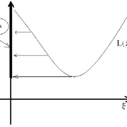
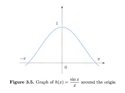
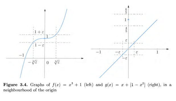
We now investigate the behaviour of the values $y=f(x)$ of a function $f$ when $x$ ‘approaches’ a point $x_0 \in \mathbb{R}$. Suppose $f$ is defined in a neighbourhood of $x_0$, but not necessarily at the point $x_0$ itself. Two examples will let us capture the essence of the notions of continuity and finite limit. Fix $x_0=0$ and consider the real functions of real variable $f(x)=x^3+1, g(x)=x+\left[1-x^2\right]$ and $h(x)=\frac{\sin x}{x}$ (recall that $[z]$ indicates the integer part of $z$ ); their respective graphs, at least in a neighbourhood of the origin, are presented in Fig. 3.4 and 3.5 .
As far as $g$ is concerned, we observe that $|x|<1$ implies $0<1-x^2 \leq 1$ and $g$ assumes the value 1 only at $x=0$; in the neighbourhood of the origin of unit radius then, $$ g(x)= \begin{cases}1 & \text { if } x=0, \ x & \text { if } x \neq 0,\end{cases} $$ as the picture shows. Note the function $h$ is not defined in the origin. For each of $f$ and $g$, let us compare the values at points $x$ near the origin with the actual value at the origin. The two functions behave rather differently. The value $f(0)=1$ can be approximated as well as we like by any $f(x)$, provided $x$ is close enough to 0 . Precisely, having fixed an (arbitrarily small) ‘error’ $\varepsilon>0$ in advance, we can make $|f(x)-f(0)|$ smaller than $\varepsilon$ for all $x$ such that $|x-0|=|x|$ is smaller than a suitable real $\delta>0$. In fact $|f(x)-f(0)|=\left|x^3\right|=|x|^3<\varepsilon$ means $|x|<\sqrt[3]{\varepsilon}$, so it is sufficient to choose $\delta=\sqrt[3]{\varepsilon}$. We shall say that the function $f$ is continuous at the origin.
On the other hand, $g(0)=1$ cannot be approximated well by any $g(x)$ with $x$ close to 0 . For instance, let $\varepsilon=\frac{1}{5}$. Then $|g(x)-g(0)|<\varepsilon$ is equivalent to $\frac{4}{5}<g(x)<\frac{6}{5}$; but all $x$ different from 0 and such that, say, $|x|<\frac{1}{2}$, satisfy $-\frac{1}{2}<g(x)=x<\frac{1}{2}$, in violation to the constraint for $g(x)$. The function $g$ is not continuous at the origin.
At any rate, we can specify the behaviour of $g$ around 0 : for $x$ closer and closer to 0 , yet different from 0 , the images $g(x)$ approximate not the value $g(0)$, but rather $\ell=0$. In fact, with $\varepsilon>0$ fixed, if $x \neq 0$ satisfies $|x|<\min (\varepsilon, 1)$, then $g(x)=x$ and $|g(x)-\ell|=|g(x)|=|x|<\varepsilon$. We say that $g$ has limit 0 for $x$ going to 0 .
As for the function $h$, it cannot be continuous at the origin, since comparing the values $h(x)$, for $x$ near 0 , with the value at the origin simply makes no sense, for the latter is not even defined. Neverthless, the graph allows to ‘conjecture’ that these values might estimate $\ell=1$ increasingly better, the closer we choose $x$ to the origin. We are lead to say $h$ has a limit for $x$ going to 0 , and this limit is 1 . We shall substantiate this claim later on.
数学分析代写
数学代写|数学分析代写MATHEMATICAL ANALYSIS代考|Limits of functions; continuity
Let $f$ be a real function of real variable. We wish to describe the behaviour of the dependent variable $y=f(x)$ when the independent variable $x$ ‘approaches’ a certain point $x_0 \in \mathbb{R}$, or one of the points at infinity $-\infty,+\infty$. We start with the latter case for conveniency, because we have already studied what sequences do at infinity.
3.3.1 Limits at infinity
Suppose $f$ is defined around $+\infty$. In analogy to sequences we have some definitions.
Definition 3.11 The function $f$ tends to the limit $\ell \in \mathbb{R}$ for $x$ going to $+\infty$, in symbols
$$
\lim _{x \rightarrow+\infty} f(x)=\ell,
$$
if for any real number $\varepsilon>0$ there is a real $B \geq 0$ such that
$$
\forall x \in \operatorname{dom} f, \quad x>B \quad \Rightarrow \quad|f(x)-\ell|<\varepsilon .
$$
This condition requires that for any neighbourhood $I_{\varepsilon}(\ell)$ of $\ell$, there exists a neighbourhood $I_B(+\infty)$ of $+\infty$ such that
$$
\forall x \in \operatorname{dom} f, \quad x \in I_B(+\infty) \quad \Rightarrow \quad f(x) \in I_{\varepsilon}(\ell) .
$$
Definition 3.12 The function $f$ tends to $+\infty$ for $x$ going to $+\infty$, in symbols
$$
\lim {x \rightarrow+\infty} f(x)=+\infty, $$ if for each real $A>0$ there is a real $B \geq 0$ such that $$ \forall x \in \operatorname{dom} f, \quad x>B \quad \Rightarrow \quad f(x)>A . $$ For functions tending to $-\infty$ one should replace $f(x)>A$ by $f(x)<-A$. The expression $$ \lim {x \rightarrow+\infty} f(x)=\infty
$$
means $\lim {x \rightarrow+\infty}|f(x)|=+\infty$. If $f$ is defined around $-\infty$, Definitions 3.11 and 3.12 modify to become definitions of limit ( $L$, finite or infinite) for $x$ going to $-\infty$, by changing $x>B$ to $x<-B$ : $$ \lim {x \rightarrow-\infty} f(x)=L
$$
At last, by
$$
\lim _{x \rightarrow \infty} f(x)=L
$$
one intends that $f$ has limit $L$ (finite or not) both for $x \rightarrow+\infty$ and $x \rightarrow-\infty$.
数学代写|数学分析代写MATHEMATICAL ANALYSIS代考|Continuity. Limits at real points
We now investigate the behaviour of the values $y=f(x)$ of a function $f$ when $x$ ‘approaches’ a point $x_0 \in \mathbb{R}$. Suppose $f$ is defined in a neighbourhood of $x_0$, but not necessarily at the point $x_0$ itself. Two examples will let us capture the essence of the notions of continuity and finite limit. Fix $x_0=0$ and consider the real functions of real variable $f(x)=x^3+1, g(x)=x+\left[1-x^2\right]$ and $h(x)=\frac{\sin x}{x}$ (recall that $[z]$ indicates the integer part of $z$ ); their respective graphs, at least in a neighbourhood of the origin, are presented in Fig. 3.4 and 3.5 .
As far as $g$ is concerned, we observe that $|x|<1$ implies $0<1-x^2 \leq 1$ and $g$ assumes the value 1 only at $x=0$; in the neighbourhood of the origin of unit radius then, $$ g(x)= \begin{cases}1 & \text { if } x=0, \ x & \text { if } x \neq 0,\end{cases} $$ as the picture shows. Note the function $h$ is not defined in the origin. For each of $f$ and $g$, let us compare the values at points $x$ near the origin with the actual value at the origin. The two functions behave rather differently. The value $f(0)=1$ can be approximated as well as we like by any $f(x)$, provided $x$ is close enough to 0 . Precisely, having fixed an (arbitrarily small) ‘error’ $\varepsilon>0$ in advance, we can make $|f(x)-f(0)|$ smaller than $\varepsilon$ for all $x$ such that $|x-0|=|x|$ is smaller than a suitable real $\delta>0$. In fact $|f(x)-f(0)|=\left|x^3\right|=|x|^3<\varepsilon$ means $|x|<\sqrt[3]{\varepsilon}$, so it is sufficient to choose $\delta=\sqrt[3]{\varepsilon}$. We shall say that the function $f$ is continuous at the origin.
On the other hand, $g(0)=1$ cannot be approximated well by any $g(x)$ with $x$ close to 0 . For instance, let $\varepsilon=\frac{1}{5}$. Then $|g(x)-g(0)|<\varepsilon$ is equivalent to $\frac{4}{5}<g(x)<\frac{6}{5}$; but all $x$ different from 0 and such that, say, $|x|<\frac{1}{2}$, satisfy $-\frac{1}{2}<g(x)=x<\frac{1}{2}$, in violation to the constraint for $g(x)$. The function $g$ is not continuous at the origin.
At any rate, we can specify the behaviour of $g$ around 0 : for $x$ closer and closer to 0 , yet different from 0 , the images $g(x)$ approximate not the value $g(0)$, but rather $\ell=0$. In fact, with $\varepsilon>0$ fixed, if $x \neq 0$ satisfies $|x|<\min (\varepsilon, 1)$, then $g(x)=x$ and $|g(x)-\ell|=|g(x)|=|x|<\varepsilon$. We say that $g$ has limit 0 for $x$ going to 0 .
As for the function $h$, it cannot be continuous at the origin, since comparing the values $h(x)$, for $x$ near 0 , with the value at the origin simply makes no sense, for the latter is not even defined. Neverthless, the graph allows to ‘conjecture’ that these values might estimate $\ell=1$ increasingly better, the closer we choose $x$ to the origin. We are lead to say $h$ has a limit for $x$ going to 0 , and this limit is 1 . We shall substantiate this claim later on.

数学代写|数学分析代写Mathematical Analysis代考 请认准UprivateTA™. UprivateTA™为您的留学生涯保驾护航。
微观经济学代写
微观经济学是主流经济学的一个分支,研究个人和企业在做出有关稀缺资源分配的决策时的行为以及这些个人和企业之间的相互作用。my-assignmentexpert™ 为您的留学生涯保驾护航 在数学Mathematics作业代写方面已经树立了自己的口碑, 保证靠谱, 高质且原创的数学Mathematics代写服务。我们的专家在图论代写Graph Theory代写方面经验极为丰富,各种图论代写Graph Theory相关的作业也就用不着 说。
线性代数代写
线性代数是数学的一个分支,涉及线性方程,如:线性图,如:以及它们在向量空间和通过矩阵的表示。线性代数是几乎所有数学领域的核心。
博弈论代写
现代博弈论始于约翰-冯-诺伊曼(John von Neumann)提出的两人零和博弈中的混合策略均衡的观点及其证明。冯-诺依曼的原始证明使用了关于连续映射到紧凑凸集的布劳威尔定点定理,这成为博弈论和数学经济学的标准方法。在他的论文之后,1944年,他与奥斯卡-莫根斯特恩(Oskar Morgenstern)共同撰写了《游戏和经济行为理论》一书,该书考虑了几个参与者的合作游戏。这本书的第二版提供了预期效用的公理理论,使数理统计学家和经济学家能够处理不确定性下的决策。
微积分代写
微积分,最初被称为无穷小微积分或 “无穷小的微积分”,是对连续变化的数学研究,就像几何学是对形状的研究,而代数是对算术运算的概括研究一样。
它有两个主要分支,微分和积分;微分涉及瞬时变化率和曲线的斜率,而积分涉及数量的累积,以及曲线下或曲线之间的面积。这两个分支通过微积分的基本定理相互联系,它们利用了无限序列和无限级数收敛到一个明确定义的极限的基本概念 。
计量经济学代写
什么是计量经济学?
计量经济学是统计学和数学模型的定量应用,使用数据来发展理论或测试经济学中的现有假设,并根据历史数据预测未来趋势。它对现实世界的数据进行统计试验,然后将结果与被测试的理论进行比较和对比。
根据你是对测试现有理论感兴趣,还是对利用现有数据在这些观察的基础上提出新的假设感兴趣,计量经济学可以细分为两大类:理论和应用。那些经常从事这种实践的人通常被称为计量经济学家。
Matlab代写
MATLAB 是一种用于技术计算的高性能语言。它将计算、可视化和编程集成在一个易于使用的环境中,其中问题和解决方案以熟悉的数学符号表示。典型用途包括:数学和计算算法开发建模、仿真和原型制作数据分析、探索和可视化科学和工程图形应用程序开发,包括图形用户界面构建MATLAB 是一个交互式系统,其基本数据元素是一个不需要维度的数组。这使您可以解决许多技术计算问题,尤其是那些具有矩阵和向量公式的问题,而只需用 C 或 Fortran 等标量非交互式语言编写程序所需的时间的一小部分。MATLAB 名称代表矩阵实验室。MATLAB 最初的编写目的是提供对由 LINPACK 和 EISPACK 项目开发的矩阵软件的轻松访问,这两个项目共同代表了矩阵计算软件的最新技术。MATLAB 经过多年的发展,得到了许多用户的投入。在大学环境中,它是数学、工程和科学入门和高级课程的标准教学工具。在工业领域,MATLAB 是高效研究、开发和分析的首选工具。MATLAB 具有一系列称为工具箱的特定于应用程序的解决方案。对于大多数 MATLAB 用户来说非常重要,工具箱允许您学习和应用专业技术。工具箱是 MATLAB 函数(M 文件)的综合集合,可扩展 MATLAB 环境以解决特定类别的问题。可用工具箱的领域包括信号处理、控制系统、神经网络、模糊逻辑、小波、仿真等。