如果你也在 怎样代写电动力学Electrodynamics 这个学科遇到相关的难题，请随时右上角联系我们的24/7代写客服。电动力学Electrodynamics研究运动中的带电体和变化的电场和磁场(参见charge;电);由于移动的电荷产生磁场，电动力学与磁学、电磁辐射和电磁感应等效应有关，包括发电机和电动机等实际应用。

电动力学Electrodynamics的这一领域，通常被称为经典电动力学，最早是由物理学家詹姆斯·克拉克·麦克斯韦系统地解释的。麦克斯韦方程组是一组微分方程，它概括地描述了这一领域的现象。最近的一个发展是量子电动力学，它被用来解释电磁辐射与物质的相互作用，量子理论的定律也适用于此。物理学家P. A. M.狄拉克、W.海森堡和W.泡利是量子电动力学公式的先驱。当所考虑的带电粒子的速度变得与光速相当时，必须进行涉及相对论的修正;这个理论的分支叫做相对论性电动力学。它适用于与粒子加速器和受高压和大电流影响的电子管有关的现象。

同学们在留学期间，都对各式各样的作业考试很是头疼，如果你无从下手，不如考虑my-assignmentexpert™！

my-assignmentexpert™提供最专业的一站式服务：Essay代写，Dissertation代写，Assignment代写，Paper代写，Proposal代写，Proposal代写，Literature Review代写，Online Course，Exam代考等等。my-assignmentexpert™专注为留学生提供Essay代写服务，拥有各个专业的博硕教师团队帮您代写，免费修改及辅导，保证成果完成的效率和质量。同时有多家检测平台帐号，包括Turnitin高级账户，检测论文不会留痕，写好后检测修改，放心可靠，经得起任何考验！

物理代写|电动力学代考Electrodynamics代写|Spherical Coordinates

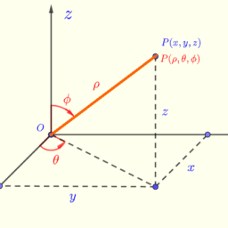
Figure 1.2(b) defines spherical coordinates $(r, \theta, \phi)$. Our notation for the components and unit vectors in this system is
$$
\mathbf{V}=V_r \hat{\mathbf{r}}+V_\theta \hat{\boldsymbol{\theta}}+V_\phi \hat{\boldsymbol{\phi}} .
$$
The transformation to Cartesian coordinates is
$$
x=r \sin \theta \cos \phi \quad y=r \sin \theta \sin \phi \quad z=r \cos \theta .
$$
The volume element in spherical coordinates is $d^3 r=r^2 \sin \theta d r d \theta d \phi$. The unit vectors are related by
$$
\begin{array}{cc}
\hat{\mathbf{r}}=\hat{\mathbf{x}} \sin \theta \cos \phi+\hat{\mathbf{y}} \sin \theta \sin \phi+\hat{\mathbf{z}} \cos \theta & \hat{\mathbf{x}}=\hat{\mathbf{r}} \sin \theta \cos \phi+\hat{\boldsymbol{\theta}} \cos \theta \cos \phi-\hat{\boldsymbol{\phi}} \sin \phi \
\hat{\boldsymbol{\theta}}=\hat{\mathbf{x}} \cos \theta \cos \phi+\hat{\mathbf{y}} \cos \theta \sin \phi-\hat{\mathbf{z}} \sin \theta & \hat{\mathbf{y}}=\hat{\mathbf{r}} \sin \theta \sin \phi+\hat{\boldsymbol{\theta}} \cos \theta \sin \phi+\hat{\boldsymbol{\phi}} \cos \phi \
\hat{\boldsymbol{\phi}}=-\hat{\mathbf{x}} \sin \phi+\hat{\mathbf{y}} \cos \phi & \hat{\mathbf{z}}=\hat{\mathbf{r}} \cos \theta-\hat{\boldsymbol{\theta}} \sin \theta .
\end{array}
$$
The gradient operator in spherical coordinates is
$$
\nabla=\hat{\mathbf{r}} \frac{\partial}{\partial r}+\frac{\hat{\boldsymbol{\theta}}}{r} \frac{\partial}{\partial \theta}+\frac{\hat{\boldsymbol{\phi}}}{r \sin \theta} \frac{\partial}{\partial \phi} .
$$
The divergence, curl, and Laplacian operations are, respectively,
$$
\begin{aligned}
\nabla \cdot \mathbf{V}= & \frac{1}{r^2} \frac{\partial\left(r^2 V_r\right)}{\partial r}+\frac{1}{r \sin \theta} \frac{\partial\left(\sin \theta V_\theta\right)}{\partial \theta}+\frac{1}{r \sin \theta} \frac{\partial V_\phi}{\partial \phi} \
\nabla \times \mathbf{V}= & \frac{1}{r \sin \theta}\left[\frac{\partial\left(\sin \theta V_\phi\right)}{\partial \theta}-\frac{\partial V_\theta}{\partial \phi}\right] \hat{\mathbf{r}} \
& +\frac{1}{r}\left[\frac{1}{\sin \theta} \frac{\partial V_r}{\partial \phi}-\frac{\partial\left(r V_\phi\right)}{\partial r}\right] \hat{\boldsymbol{\theta}}+\frac{1}{r}\left[\frac{\partial\left(r V_\theta\right)}{\partial r}-\frac{\partial V_r}{\partial \theta}\right] \hat{\boldsymbol{\phi}} \
\nabla^2 A= & \frac{1}{r^2} \frac{\partial}{\partial r}\left(r^2 \frac{\partial A}{\partial r}\right)+\frac{1}{r^2 \sin \theta} \frac{\partial}{\partial \theta}\left(\sin \theta \frac{\partial A}{\partial \theta}\right)+\frac{1}{r^2 \sin ^2 \theta} \frac{\partial^2 A}{\partial \phi^2} .
\end{aligned}
$$

物理代写|电动力学代考Electrodynamics代写|The Einstein Summation Convention

Einstein (1916) introduced the following convention. An index which appears exactly twice in a mathematical expression is implicitly summed over all possible values for that index. The range of this dummy index must be clear from context and the index cannot be used elsewhere in the same expression for another purpose. In this book, the range for a roman index like $i$ is from 1 to 3 , indicating a sum over the Cartesian indices $x, y$, and $z$. Thus, $\mathbf{V}$ in (1.6) and its dot product with another vector $\mathbf{F}$ are written
$$
\mathbf{V}=\sum_{k=1}^3 V_k \hat{\mathbf{e}}k \equiv V_k \hat{\mathbf{e}}_k \quad \mathbf{V} \cdot \mathbf{F}=\sum{k=1}^3 V_k F_k \equiv V_k F_k .
$$
In a Cartesian basis, the gradient of a scalar $\varphi$ and the divergence of a vector $\mathbf{D}$ can be variously written
$$
\begin{aligned}
& \nabla \varphi=\hat{\mathbf{e}}k \nabla_k \varphi=\hat{\mathbf{e}}_k \partial_k \varphi=\hat{\mathbf{e}}_k \frac{\partial \varphi}{\partial r_k} \ & \nabla \cdot \mathbf{D}=\nabla_k D_k=\partial_k D_k=\frac{\partial D_k}{\partial r_k} . \end{aligned} $$ If an $N \times N$ matrix $\mathbf{C}$ is the product of an $N \times M$ matrix $\mathbf{A}$ and an $M \times N$ matrix $\mathbf{B}$, $$ C{i k}=\sum_{j=1}^M A_{i j} B_{j k}=A_{i j} B_{j k}
$$

The Kronecker delta symbol $\delta_{i j}$ and Levi-Cività permutation symbol $\epsilon_{i j k}$ have roman indices $i, j$, and $k$ which take on the Cartesian coordinate values $x, y$, and $z$. They are defined by
$$
\delta_{i j}= \begin{cases}1 & i=j \ 0 & i \neq j\end{cases}
$$
and
$$
\epsilon_{i j k}= \begin{cases}1 & i j k=x y z \quad y z x \quad z x y, \ -1 & i j k=x z y \text { yxz } z y x, \ 0 & \text { otherwise. }\end{cases}
$$
Some useful Kronecker delta and Levi-Cività symbol identities are
$$
\begin{aligned}
\hat{\mathbf{e}}i \cdot \hat{\mathbf{e}}_j=\delta{i j} & \delta_{k k}=3 \
\partial_k r_j=\delta_{j k} & V_k \delta_{k j}=V_j \
{[\mathbf{V} \times \mathbf{F}]i=\epsilon{i j k} V_j F_k } & {[\nabla \times \mathbf{A}]i=\epsilon{i j k} \partial_j A_k } \
\delta_{i j} \epsilon_{i j k}=0 & \epsilon_{i j k} \epsilon_{i j k}=6 .
\end{aligned}
$$
A particularly useful identity involves a single sum over the repeated index $i$ :
$$
\epsilon_{i j k} \epsilon_{i s t}=\delta_{j s} \delta_{k t}-\delta_{j t} \delta_{k s} .
$$
A generalization of (1.39) when there are no repeated indices to sum over is the determinant
$$
\epsilon_{k i \ell} \epsilon_{m p q}=\left|\begin{array}{lll}
\delta_{k m} & \delta_{i m} & \delta_{\ell m} \
\delta_{k p} & \delta_{i p} & \delta_{\ell p} \
\delta_{k q} & \delta_{i q} & \delta_{\ell q}
\end{array}\right| .
$$

电动力学代写

物理代写|电动力学代考Electrodynamics代写|Spherical Coordinates

图1.2(b)定义了球坐标$(r, \theta, \phi)$。这个系统中的分量和单位向量的符号是
$$
\mathbf{V}=V_r \hat{\mathbf{r}}+V_\theta \hat{\boldsymbol{\theta}}+V_\phi \hat{\boldsymbol{\phi}} .
$$
到笛卡尔坐标的变换是
$$
x=r \sin \theta \cos \phi \quad y=r \sin \theta \sin \phi \quad z=r \cos \theta .
$$
球坐标下的体积元是$d^3 r=r^2 \sin \theta d r d \theta d \phi$。单位向量是由
$$
\begin{array}{cc}
\hat{\mathbf{r}}=\hat{\mathbf{x}} \sin \theta \cos \phi+\hat{\mathbf{y}} \sin \theta \sin \phi+\hat{\mathbf{z}} \cos \theta & \hat{\mathbf{x}}=\hat{\mathbf{r}} \sin \theta \cos \phi+\hat{\boldsymbol{\theta}} \cos \theta \cos \phi-\hat{\boldsymbol{\phi}} \sin \phi \
\hat{\boldsymbol{\theta}}=\hat{\mathbf{x}} \cos \theta \cos \phi+\hat{\mathbf{y}} \cos \theta \sin \phi-\hat{\mathbf{z}} \sin \theta & \hat{\mathbf{y}}=\hat{\mathbf{r}} \sin \theta \sin \phi+\hat{\boldsymbol{\theta}} \cos \theta \sin \phi+\hat{\boldsymbol{\phi}} \cos \phi \
\hat{\boldsymbol{\phi}}=-\hat{\mathbf{x}} \sin \phi+\hat{\mathbf{y}} \cos \phi & \hat{\mathbf{z}}=\hat{\mathbf{r}} \cos \theta-\hat{\boldsymbol{\theta}} \sin \theta .
\end{array}
$$
球坐标下的梯度算子为
$$
\nabla=\hat{\mathbf{r}} \frac{\partial}{\partial r}+\frac{\hat{\boldsymbol{\theta}}}{r} \frac{\partial}{\partial \theta}+\frac{\hat{\boldsymbol{\phi}}}{r \sin \theta} \frac{\partial}{\partial \phi} .
$$
散度，旋度和拉普拉斯运算分别是，
$$
\begin{aligned}
\nabla \cdot \mathbf{V}= & \frac{1}{r^2} \frac{\partial\left(r^2 V_r\right)}{\partial r}+\frac{1}{r \sin \theta} \frac{\partial\left(\sin \theta V_\theta\right)}{\partial \theta}+\frac{1}{r \sin \theta} \frac{\partial V_\phi}{\partial \phi} \
\nabla \times \mathbf{V}= & \frac{1}{r \sin \theta}\left[\frac{\partial\left(\sin \theta V_\phi\right)}{\partial \theta}-\frac{\partial V_\theta}{\partial \phi}\right] \hat{\mathbf{r}} \
& +\frac{1}{r}\left[\frac{1}{\sin \theta} \frac{\partial V_r}{\partial \phi}-\frac{\partial\left(r V_\phi\right)}{\partial r}\right] \hat{\boldsymbol{\theta}}+\frac{1}{r}\left[\frac{\partial\left(r V_\theta\right)}{\partial r}-\frac{\partial V_r}{\partial \theta}\right] \hat{\boldsymbol{\phi}} \
\nabla^2 A= & \frac{1}{r^2} \frac{\partial}{\partial r}\left(r^2 \frac{\partial A}{\partial r}\right)+\frac{1}{r^2 \sin \theta} \frac{\partial}{\partial \theta}\left(\sin \theta \frac{\partial A}{\partial \theta}\right)+\frac{1}{r^2 \sin ^2 \theta} \frac{\partial^2 A}{\partial \phi^2} .
\end{aligned}
$$

物理代写|电动力学代考Electrodynamics代写|The Einstein Summation Convention

爱因斯坦(1916)介绍了以下惯例。在数学表达式中恰好出现两次的索引将隐式地对该索引的所有可能值求和。这个虚拟索引的范围必须与上下文清晰，并且索引不能在同一表达式的其他地方用于其他目的。在本书中，像$i$这样的罗马索引的范围是从1到3，表示笛卡尔索引$x, y$和$z$的总和。因此，(1.6)中的$\mathbf{V}$和它与另一个向量$\mathbf{F}$的点积被写成
$$
\mathbf{V}=\sum_{k=1}^3 V_k \hat{\mathbf{e}}k \equiv V_k \hat{\mathbf{e}}k \quad \mathbf{V} \cdot \mathbf{F}=\sum{k=1}^3 V_k F_k \equiv V_k F_k . $$ 在笛卡尔基中，标量的梯度$\varphi$和矢量的散度$\mathbf{D}$可以写成不同的形式 $$ \begin{aligned} & \nabla \varphi=\hat{\mathbf{e}}k \nabla_k \varphi=\hat{\mathbf{e}}_k \partial_k \varphi=\hat{\mathbf{e}}_k \frac{\partial \varphi}{\partial r_k} \ & \nabla \cdot \mathbf{D}=\nabla_k D_k=\partial_k D_k=\frac{\partial D_k}{\partial r_k} . \end{aligned} $$如果$N \times N$矩阵$\mathbf{C}$是$N \times M$矩阵$\mathbf{A}$和$M \times N$矩阵$\mathbf{B}$的乘积， $$ C{i k}=\sum{j=1}^M A_{i j} B_{j k}=A_{i j} B_{j k}
$$

克罗内克符号$\delta_{i j}$和列维-齐维特排列符号$\epsilon_{i j k}$具有罗马指标$i, j$和$k$，它们采用笛卡尔坐标值$x, y$和$z$。它们的定义是
$$
\delta_{i j}= \begin{cases}1 & i=j \ 0 & i \neq j\end{cases}
$$
和
$$
\epsilon_{i j k}= \begin{cases}1 & i j k=x y z \quad y z x \quad z x y, \ -1 & i j k=x z y \text { yxz } z y x, \ 0 & \text { otherwise. }\end{cases}
$$
一些有用的克罗内克符号恒等式和列维符号恒等式是
$$
\begin{aligned}
\hat{\mathbf{e}}i \cdot \hat{\mathbf{e}}j=\delta{i j} & \delta{k k}=3 \
\partial_k r_j=\delta_{j k} & V_k \delta_{k j}=V_j \
{[\mathbf{V} \times \mathbf{F}]i=\epsilon{i j k} V_j F_k } & {[\nabla \times \mathbf{A}]i=\epsilon{i j k} \partial_j A_k } \
\delta_{i j} \epsilon_{i j k}=0 & \epsilon_{i j k} \epsilon_{i j k}=6 .
\end{aligned}
$$
一个特别有用的恒等式涉及对重复索引$i$的单个求和:
$$
\epsilon_{i j k} \epsilon_{i s t}=\delta_{j s} \delta_{k t}-\delta_{j t} \delta_{k s} .
$$
当没有重复指标需要求和时，式(1.39)的概化就是行列式
$$
\epsilon_{k i \ell} \epsilon_{m p q}=\left|\begin{array}{lll}
\delta_{k m} & \delta_{i m} & \delta_{\ell m} \
\delta_{k p} & \delta_{i p} & \delta_{\ell p} \
\delta_{k q} & \delta_{i q} & \delta_{\ell q}
\end{array}\right| .
$$

物理代写|电动力学代考Electrodynamics代写 请认准exambang™. exambang™为您的留学生涯保驾护航。

微观经济学代写

微观经济学是主流经济学的一个分支，研究个人和企业在做出有关稀缺资源分配的决策时的行为以及这些个人和企业之间的相互作用。my-assignmentexpert™ 为您的留学生涯保驾护航 在数学Mathematics作业代写方面已经树立了自己的口碑, 保证靠谱, 高质且原创的数学Mathematics代写服务。我们的专家在图论代写Graph Theory代写方面经验极为丰富，各种图论代写Graph Theory相关的作业也就用不着 说。

线性代数代写

线性代数是数学的一个分支，涉及线性方程，如：线性图，如：以及它们在向量空间和通过矩阵的表示。线性代数是几乎所有数学领域的核心。

博弈论代写

现代博弈论始于约翰-冯-诺伊曼（John von Neumann）提出的两人零和博弈中的混合策略均衡的观点及其证明。冯-诺依曼的原始证明使用了关于连续映射到紧凑凸集的布劳威尔定点定理，这成为博弈论和数学经济学的标准方法。在他的论文之后，1944年，他与奥斯卡-莫根斯特恩（Oskar Morgenstern）共同撰写了《游戏和经济行为理论》一书，该书考虑了几个参与者的合作游戏。这本书的第二版提供了预期效用的公理理论，使数理统计学家和经济学家能够处理不确定性下的决策。

微积分代写

微积分，最初被称为无穷小微积分或 “无穷小的微积分”，是对连续变化的数学研究，就像几何学是对形状的研究，而代数是对算术运算的概括研究一样。

它有两个主要分支，微分和积分；微分涉及瞬时变化率和曲线的斜率，而积分涉及数量的累积，以及曲线下或曲线之间的面积。这两个分支通过微积分的基本定理相互联系，它们利用了无限序列和无限级数收敛到一个明确定义的极限的基本概念 。

计量经济学代写

什么是计量经济学？
计量经济学是统计学和数学模型的定量应用，使用数据来发展理论或测试经济学中的现有假设，并根据历史数据预测未来趋势。它对现实世界的数据进行统计试验，然后将结果与被测试的理论进行比较和对比。

根据你是对测试现有理论感兴趣，还是对利用现有数据在这些观察的基础上提出新的假设感兴趣，计量经济学可以细分为两大类：理论和应用。那些经常从事这种实践的人通常被称为计量经济学家。

Matlab代写

MATLAB 是一种用于技术计算的高性能语言。它将计算、可视化和编程集成在一个易于使用的环境中，其中问题和解决方案以熟悉的数学符号表示。典型用途包括：数学和计算算法开发建模、仿真和原型制作数据分析、探索和可视化科学和工程图形应用程序开发，包括图形用户界面构建MATLAB 是一个交互式系统，其基本数据元素是一个不需要维度的数组。这使您可以解决许多技术计算问题，尤其是那些具有矩阵和向量公式的问题，而只需用 C 或 Fortran 等标量非交互式语言编写程序所需的时间的一小部分。MATLAB 名称代表矩阵实验室。MATLAB 最初的编写目的是提供对由 LINPACK 和 EISPACK 项目开发的矩阵软件的轻松访问，这两个项目共同代表了矩阵计算软件的最新技术。MATLAB 经过多年的发展，得到了许多用户的投入。在大学环境中，它是数学、工程和科学入门和高级课程的标准教学工具。在工业领域，MATLAB 是高效研究、开发和分析的首选工具。MATLAB 具有一系列称为工具箱的特定于应用程序的解决方案。对于大多数 MATLAB 用户来说非常重要，工具箱允许您学习和应用专业技术。工具箱是 MATLAB 函数（M 文件）的综合集合，可扩展 MATLAB 环境以解决特定类别的问题。可用工具箱的领域包括信号处理、控制系统、神经网络、模糊逻辑、小波、仿真等。