如果你也在 怎样代写固体物理Solid Physics PHYS7635 PHY360这个学科遇到相关的难题,请随时右上角联系我们的24/7代写客服。固体物理Solid Physics是通过量子力学、晶体学、电磁学和冶金学等方法研究刚性物质或固体。它是凝聚态物理学的最大分支。固体物理学研究固体材料的大尺度特性是如何产生于其原子尺度特性的。因此,固态物理学构成了材料科学的理论基础。它也有直接的应用,例如在晶体管和半导体的技术中。
固体物理Solid Physics是由密密麻麻的原子形成的,这些原子之间有强烈的相互作用。这些相互作用产生了固体的机械(如硬度和弹性)、热、电、磁和光学特性。根据所涉及的材料及其形成的条件,原子可能以有规律的几何模式排列(晶体固体,包括金属和普通水冰)或不规则地排列(非晶体固体,如普通窗玻璃)。
my-assignmentexpert™固体物理Solid Physics代写,免费提交作业要求, 满意后付款,成绩80\%以下全额退款,安全省心无顾虑。专业硕 博写手团队,所有订单可靠准时,保证 100% 原创。my-assignmentexpert™, 最高质量的固体物理Solid Physics作业代写,服务覆盖北美、欧洲、澳洲等 国家。 在代写价格方面,考虑到同学们的经济条件,在保障代写质量的前提下,我们为客户提供最合理的价格。 由于统计Statistics作业种类很多,同时其中的大部分作业在字数上都没有具体要求,因此固体物理Solid Physics作业代写的价格不固定。通常在经济学专家查看完作业要求之后会给出报价。作业难度和截止日期对价格也有很大的影响。
想知道您作业确定的价格吗? 免费下单以相关学科的专家能了解具体的要求之后在1-3个小时就提出价格。专家的 报价比上列的价格能便宜好几倍。
my-assignmentexpert™ 为您的留学生涯保驾护航 在物理Physics代写方面已经树立了自己的口碑, 保证靠谱, 高质且原创的物理Physics代写服务。我们的专家在固体物理Solid Physics代写方面经验极为丰富,各种固体物理Solid Physics相关的作业也就用不着 说。
我们提供的固体物理Solid Physics 及其相关学科的代写,服务范围广, 其中包括但不限于:
物理代写|固体物理代写Solid Physics代考|Electron dynamics
It is very convenient to address electron dynamics within a semi-classical scheme according to which: (i) electron energy states are described quantum mechanically, but (ii) their equations of motion are classical. This approximated scheme is trustworthy when one wants to study the motion of the electrons over a length scale much larger than the interatomic distances. This is, for instance, the relevant case of motion under the action of an externally applied and slowly varying electric field, that is an electric field which is practically constant over the length scale of interatomic lattice distances. On the other hand, the results of this approximation can hardly be extended to the case of nanostructures $[16,17]$, that is to solid state systems whose structural features display on the $10^{-9} \mathrm{~m}$ scale: here a full quantum theory of electron transport is needed, as detailed elsewhere [12, 17-19].
Let us at first consider the dynamics of an electron in the absence of an external electric field. If it is accommodated on the $n$th band, then its velocity $v_n(k)$ is given by the group velocity of the corresponding matter wave
$$
v_n(k)=\frac{d \omega_n(k)}{d k}=\frac{1}{\hbar} \frac{d E_n(k)}{d k},
$$
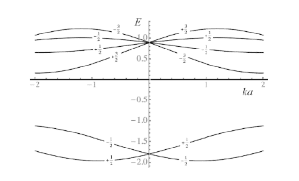
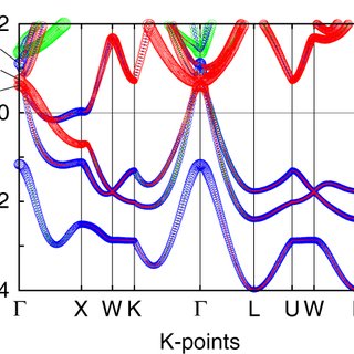
where of course we used the $E_n(k)=\hbar \omega_n(k)$ matter-wave duality relation. This result is as much mathematically straightforward as it is dense in physical implications: the velocity depends on electron wavevector and the kind of band on which the electron is accommodated. In other words, electrons with identical wavevector, but belonging to different bands, have different velocity; equation (8.29) indicates that their velocity is calculated as the angular coefficient of the band tangent at the selected $k$-point. Similarly, an electron accommodated on a given band will have different velocity depending on its wavevector. Incidentally, this is one of the most important reasons why it is so necessary to know in detail the band structure of a solid: our ability to correctly describe the electron dynamics ultimately depends on $\mathrm{it}^{13}$. In any case, this result indeed represents a major conceptual difference with respect to a pure free electron theory, where just the same (average) drift or thermal velocity was attached to each electron. Another intriguing feature is that a VB electron and a CB electron with the same wavevector move in opposite directions, as clearly understood by inspection of figure 8.6: indeed an unexpected result which, as soon to be explained, has many implications in the theory of charge transport mediated by electrons subject to a periodic crystal field potential.
In the one-dimensional case the calculation of the electron velocity is easy: simply, we must combine equation (8.29) with equations (8.20) and (8.21) to obtain the results summarised in figure 8.9. Interestingly enough, this simple case illustrates quite an important new feature, namely: once a band is selected, it is possible that an electron placed there has zero velocity (this corresponds to a zone-centre or zoneboundary wavevector) and it also moves in both possible directions, depending on its wavevector (in a one-dimensional system, it can move both to the right and to the left).
物理代写|固体物理代写Solid Physics代考|Electric field effects
Let us now apply a constant and uniform electric field $\mathbf{E}$ along a one-dimensional crystal. Within the semi-classical scheme a driving force
$$
F=-e|\mathbf{E}|=\hbar \frac{d k}{d t},
$$
is calculated, governing the drift motion of the electron. The solution of this equation of motion is
$$
k(t)=k_0-\frac{e|\mathbf{E}|}{\hbar} t,
$$
where $k_0$ is the electron wavevector at time $t=0$, that is, when the electric field is turned on. By making use of equation (8.29) this result reflects in a time-dependent electron velocity
$$
v_n(k, t)=\frac{1}{\hbar} \frac{d E_n}{d k(t)},
$$
suggesting the practical rule that under the action of an electric field, the electron velocity at time $t$ is calculated by evaluating the slope of band tangent at the point $k(t)$ given in equation (8.32). This result has a quite interesting implication, as we easily understand by considering the case of an electron in the valence band: under the action of the electric field, which we consider oriented to the left with no loss of generality, the wavevector varies linearly with time, assuming gradually increasing values and, therefore, it will sooner or later end up reaching the right edge of the 1BZ. However, given the crystalline periodicity, the $k=+\pi / a$ value defines a quantum state equivalent to the one described by $k^{\prime}=k+G$ with $G=-2 \pi / a$ a reciprocal lattice vector. This is tantamount to saying that the electron, once it reaches the right edge, is flipped back to a state corresponding the left one. Next, as time goes by, the electron will again assume increasing wavevector values, as before eventually reaching the right edge of $1 \mathrm{BZ}$ : here its wavevector will be flipped back once more. And so on … This periodic back-and-forth variation of $k(t)$ in the Brillouin zone will continue as long as the electric field is present. This phenomenon is described by saying that under the action of an electric field a band electron is subjected to Bloch oscillations: their graphical rendering is reported in figure 8.10.
固体物理代写
物理代写|固体物理代写固体物理学代考|电子动力学
在半经典格式中处理电子动力学问题是非常方便的,根据这种格式:(i)电子能态是用量子力学描述的,但(ii)它们的运动方程是经典的。当人们想要研究电子在比原子间距离大得多的长度尺度上的运动时,这种近似方案是值得信赖的。这是,举个例子,在一个外部作用的缓慢变化的电场作用下运动的相关情况,这个电场在原子间晶格距离的长度范围内实际上是恒定的。另一方面,这种近似的结果很难扩展到纳米结构$[16,17]$的情况,也就是说,其结构特征在$10^{-9} \mathrm{~m}$尺度上显示的固态系统:在这里,需要一个完整的电子输运量子理论,如别处所详述[12,17 -19]
让我们首先考虑在没有外电场的情况下电子的动力学。如果它被容纳在$n$波段,那么它的速度$v_n(k)$由相应物质波的群速度
$$
v_n(k)=\frac{d \omega_n(k)}{d k}=\frac{1}{\hbar} \frac{d E_n(k)}{d k},
$$
给出,当然我们使用$E_n(k)=\hbar \omega_n(k)$物质波对偶关系。这个结果在数学上很直接,在物理意义上也很丰富:速度取决于电子波矢和电子所容纳的带的种类。换句话说,波矢相同但属于不同波段的电子速度不同;式(8.29)表明,它们的速度计算为所选$k$点的带切角系数。同样,在给定波段上的电子,其速度也会因其波矢而异。顺便说一下,这也是为什么我们有必要详细了解固体的能带结构的最重要的原因之一:我们正确描述电子动力学的能力最终取决于$\mathrm{it}^{13}$。在任何情况下,这一结果确实代表了与纯自由电子理论的一个主要概念差异,在纯自由电子理论中,每个电子都附加相同的(平均)漂移或热速度。另一个有趣的特征是,具有相同波矢的VB电子和CB电子向相反的方向移动,这一点通过观察图8.6就能清楚地理解:这确实是一个意想不到的结果,很快就会解释,它对受周期性晶体场势影响的电子所调节的电荷输运理论有许多含义
在一维情况下,电子速度的计算很容易:简单地说,我们必须将式(8.29)与式(8.20)和式(8.21)结合起来,才能得到图8.9所总结的结果。有趣的是,这个简单的例子说明了一个相当重要的新特征,即:一旦选择了一个波段,放置在那里的电子有可能速度为零(这对应于一个区域中心或区域边界波矢),它也可以向两个可能的方向移动,取决于它的波矢(在一维系统中,它可以向右或向左移动)
物理代写|固体物理代写固体物理学代考|电场效应
现在让我们沿着一维晶体施加恒定均匀的电场$\mathbf{E}$。在半经典格式中,计算出控制电子漂移运动的驱动力
$$
F=-e|\mathbf{E}|=\hbar \frac{d k}{d t},
$$
。这个运动方程的解是
$$
k(t)=k_0-\frac{e|\mathbf{E}|}{\hbar} t,
$$
其中$k_0$是电子波矢量在$t=0$时刻,也就是说,当电场打开时。利用(8.29)式,该结果反映在一个随时间变化的电子速度
$$
v_n(k, t)=\frac{1}{\hbar} \frac{d E_n}{d k(t)},
$$
表示在电场作用下,电子在$t$时刻的速度通过计算式(8.32)中所示$k(t)$点的带切线斜率来计算。这个结果有一个非常有趣的含义,我们可以通过考虑价带中的电子的情况来很容易地理解:在电场的作用下,我们认为电场是向左的,没有丧失普遍性,波矢随时间线性变化,假设值逐渐增加,因此,它迟早会到达1BZ的右边缘。然而,考虑到晶体的周期性,$k=+\pi / a$值定义了一个等价于$k^{\prime}=k+G$描述的量子态,$G=-2 \pi / a$是一个倒易晶格向量。这就等于说,电子一旦到达右边缘,就会翻转回到左边缘对应的状态。接下来,随着时间的推移,电子将再次获得不断增加的波向值,就像之前最终到达$1 \mathrm{BZ}$的右边缘一样:在这里,它的波向将再次翻转回来。只要电场存在,$k(t)$在布里渊区的这种周期性的来回变化就会继续下去。这种现象是这样描述的:在电场的作用下,带电子受到布洛赫振荡:它们的图形绘制见图8.10

物理代写|固体物理代写Solid Physics代考 请认准UprivateTA™. UprivateTA™为您的留学生涯保驾护航。
微观经济学代写
微观经济学是主流经济学的一个分支,研究个人和企业在做出有关稀缺资源分配的决策时的行为以及这些个人和企业之间的相互作用。my-assignmentexpert™ 为您的留学生涯保驾护航 在数学Mathematics作业代写方面已经树立了自己的口碑, 保证靠谱, 高质且原创的数学Mathematics代写服务。我们的专家在图论代写Graph Theory代写方面经验极为丰富,各种图论代写Graph Theory相关的作业也就用不着 说。
线性代数代写
线性代数是数学的一个分支,涉及线性方程,如:线性图,如:以及它们在向量空间和通过矩阵的表示。线性代数是几乎所有数学领域的核心。
博弈论代写
现代博弈论始于约翰-冯-诺伊曼(John von Neumann)提出的两人零和博弈中的混合策略均衡的观点及其证明。冯-诺依曼的原始证明使用了关于连续映射到紧凑凸集的布劳威尔定点定理,这成为博弈论和数学经济学的标准方法。在他的论文之后,1944年,他与奥斯卡-莫根斯特恩(Oskar Morgenstern)共同撰写了《游戏和经济行为理论》一书,该书考虑了几个参与者的合作游戏。这本书的第二版提供了预期效用的公理理论,使数理统计学家和经济学家能够处理不确定性下的决策。
微积分代写
微积分,最初被称为无穷小微积分或 “无穷小的微积分”,是对连续变化的数学研究,就像几何学是对形状的研究,而代数是对算术运算的概括研究一样。
它有两个主要分支,微分和积分;微分涉及瞬时变化率和曲线的斜率,而积分涉及数量的累积,以及曲线下或曲线之间的面积。这两个分支通过微积分的基本定理相互联系,它们利用了无限序列和无限级数收敛到一个明确定义的极限的基本概念 。
计量经济学代写
什么是计量经济学?
计量经济学是统计学和数学模型的定量应用,使用数据来发展理论或测试经济学中的现有假设,并根据历史数据预测未来趋势。它对现实世界的数据进行统计试验,然后将结果与被测试的理论进行比较和对比。
根据你是对测试现有理论感兴趣,还是对利用现有数据在这些观察的基础上提出新的假设感兴趣,计量经济学可以细分为两大类:理论和应用。那些经常从事这种实践的人通常被称为计量经济学家。
Matlab代写
MATLAB 是一种用于技术计算的高性能语言。它将计算、可视化和编程集成在一个易于使用的环境中,其中问题和解决方案以熟悉的数学符号表示。典型用途包括:数学和计算算法开发建模、仿真和原型制作数据分析、探索和可视化科学和工程图形应用程序开发,包括图形用户界面构建MATLAB 是一个交互式系统,其基本数据元素是一个不需要维度的数组。这使您可以解决许多技术计算问题,尤其是那些具有矩阵和向量公式的问题,而只需用 C 或 Fortran 等标量非交互式语言编写程序所需的时间的一小部分。MATLAB 名称代表矩阵实验室。MATLAB 最初的编写目的是提供对由 LINPACK 和 EISPACK 项目开发的矩阵软件的轻松访问,这两个项目共同代表了矩阵计算软件的最新技术。MATLAB 经过多年的发展,得到了许多用户的投入。在大学环境中,它是数学、工程和科学入门和高级课程的标准教学工具。在工业领域,MATLAB 是高效研究、开发和分析的首选工具。MATLAB 具有一系列称为工具箱的特定于应用程序的解决方案。对于大多数 MATLAB 用户来说非常重要,工具箱允许您学习和应用专业技术。工具箱是 MATLAB 函数(M 文件)的综合集合,可扩展 MATLAB 环境以解决特定类别的问题。可用工具箱的领域包括信号处理、控制系统、神经网络、模糊逻辑、小波、仿真等。