物理代写| TThe Perihelion Shift in the Orbit of Mercury 相对论代考代写 - 代考代写：100%准时可靠您的作业代写专家

0 0

By admin Physics代写数学代写物理物理代写相对论代写 2022年3月1日

代写隐藏

1 物理代写| The Perihelion Shift in the Orbit of Mercury 相对论代考

物理代写| The Perihelion Shift in the Orbit of Mercury 相对论代考

物理代写

7.3 The Perihelion Shift in the Orbit of Mercury
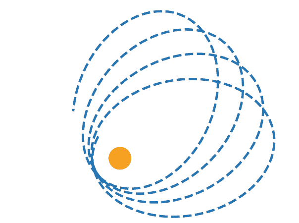
In Newton’s theory a test particle orbit is a conic section-an ellipse, a hyperbola or a parabola. If the orbit is bound as in the case of planetary motion, then the planet must describe an ellipse (in the absence of other perturbing forces). It was found that the orbit of Mercury is a precessing ellipse. Surely, there are other planets orbiting the Sun which are responsible in part for the precession, but not all of the precession could be explained away. The discrepancy not accounted for is minute-about 43 arc seconds per century. Although the discrepancy is minute, it cannot be denied. It was a great triumph for GR that it could exactly explain this discrepancy and GR became a theory to be reckoned with. Figure $7.2$ shows a precessing elliptical orbit with the sun (orange disc) at the focus. The orbit is not closed. The precession has been grossly exaggerated for clarity. In this subsection we will establish this result.
We begin with Eqs. (6.4.9) and (6.4.10), then divide one by the other to obtain the following equation:
$$
\frac{1}{r^{4}}\left(\frac{d r}{d \phi}\right)^{2}=\frac{E^{2}-1}{L^{2}}+\frac{2 m}{r}\left(\frac{1}{r^{2}}+\frac{1}{L^{2}}\right)-\frac{1}{r^{2}}
$$
Changing the variable to $u=1 / r$ as before results in,
$$
\left(\frac{d u}{d \phi}\right)^{2}+u^{2}=\frac{E^{2}-1}{L^{2}}+2 m u\left(u^{2}+\frac{1}{L^{2}}\right)
$$
This is however somewhat an inconvenient equation. A simpler equation is obtained on differentiating this equation:
$$
u^{\prime \prime}+u=\frac{m}{L^{2}}+3 m u^{2}
$$
where in the above equation we have used a short hand notation by denoting differentiation with respect to $\phi$ with a prime.

Let us now pause and understand the magnitude of the terms in Eq. (7.3.3) for Mercury’s orbit. If one ignores the second term in this equation on the RHS, this equation describes just the Newtonian orbit. The quantity $L$-angular momentum per unit rest mass at infinity-is just the Newtnonian angular momentum $L_{N} / c$. This is evident from Eq. (6.4.9) in which the differentiation is with respect to $s$ which
Fig. 7.2 The figure depicts a precessing elliptical orbit with the sun (orange disc) at the focus. The orbit is not closed. The precession has been grossly exaggerated for clarity
is the proper time multiplied by $c$ or $d s=c d \tau$. But since the velocity of Mercury is small compared with $c, d s \approx c d t$. This brings in the factor $c$ or $L_{N}=c L$. The Newtonian equation is,
$$
u^{\prime \prime}+u=\frac{m}{L^{2}}=\frac{G M}{L_{N}^{2}} \equiv \frac{1}{l}
$$
where $l$ is the latus rectum. This equation has the solution:
$$
u=\frac{1}{l}(1+e \cos \phi)
$$
Eq. (7.3.5) is the Newtonian solution for the orbit. $e$ is the eccentricity of Mercury’s orbit and it is reasonably small so that the orbit can be considered to be roughly circular. Then $l \sim$ radius of the orbit $\sim 6 \times 10^{7} \mathrm{~km}$. Now going back to Eq. (7.3.3) we can see that the second term on the RHS is $\sim 3 m / l^{2}$ because $u \sim 1 / l$ while the first term is $1 / l$. Thus the second term is smaller by a factor of $3 m / l \sim 10^{-7}$ as compared to the first. Recall that the Sun’s mass $m \sim 1.5 \mathrm{~km}$. It is therefore a small perturbation of the orbit and therefore it has an extremely small effect. The essential effect we are interested in is the precession of the elliptical orbit.
7 Classical Tests of General Relativity
126
Let us therefore write the total solution as $u=u_{0}+u_{1}$, where $u_{0}$ is the Newtonian solution given in Eq. (7.3.5). Then to the first order $u_{1}$ satisfies the equation:
$$
\begin{aligned}
u_{1}^{\prime \prime}+u_{1} &=3 m u_{0}^{2} \
&=\frac{3 m}{l^{2}}\left(1+2 e \cos \phi+e^{2} \cos ^{2} \phi\right)
\end{aligned}
$$
We remark that the perturbation scheme can be carried out in a systematic way just as we did for the case of deflection of light by the Sun. We could have defined $v=l u$ and written the full equation as $v^{\prime \prime}+v=1+\epsilon v^{2}$, where $\epsilon=3 m / l$, then separated out the equation at orders 0 and 1 of $\epsilon$. Carrying out these steps, we would have obtained identical results.

There are now three terms on the RHS of Eq. (7.3.6). The first and third term, that is the constant term and the $\cos ^{2} \phi$ term only produce a bounded oscillatory solution. It is the term in $\cos \phi$ which is responsible for a secular increase in phase and hence for precession of the orbit. Therefore, taking only this term into account, we find that the solution is,
$$
u_{1}=\frac{3 m e}{l^{2}} \phi \sin \phi
$$
The above solution can be easily verified by direct substitution. The full solution is,
$$
\begin{aligned}
u &=\frac{1}{l}(1+e \cos \phi)+\frac{3 m e}{l^{2}} \phi \sin \phi \
&=\frac{1}{l}[1+e(\cos \phi+\delta \sin \phi)]
\end{aligned}
$$
where,
$$
\delta=\frac{3 m}{l} \phi
$$

物理代考

7.3 水星轨道的近日点位移
在牛顿的理论中，测试粒子的轨道是一个圆锥截面——椭圆、双曲线或抛物线。如果轨道像行星运动一样是有界的，那么行星必须描述一个椭圆（在没有其他扰动力的情况下）。发现水星的轨道是一个进动椭圆。当然，还有其他绕太阳运行的行星对岁差负有部分责任，但并不是所有的岁差都可以被解释掉。没有考虑到的差异是分钟——大约每世纪 43 角秒。尽管差异很小，但不能否认。对于 GR 来说，这是一个巨大的胜利，它可以准确地解释这种差异，并且 GR 成为一个不可忽视的理论。图 $7.2$ 显示了一个进动椭圆轨道，太阳（橙色圆盘）位于焦点处。轨道不是封闭的。为了清楚起见，岁差被严重夸大了。在本小节中，我们将建立这个结果。
我们从方程式开始。 (6.4.9) 和 (6.4.10)，然后一个除以另一个，得到以下等式：
$$
\frac{1}{r^{4}}\left(\frac{dr}{d \phi}\right)^{2}=\frac{E^{2}-1}{L^{2} }+\frac{2 m}{r}\left(\frac{1}{r^{2}}+\frac{1}{L^{2}}\right)-\frac{1}{r ^{2}}
$$
像以前一样将变量更改为 $u=1 / r$ 会导致，
$$
\left(\frac{du}{d \phi}\right)^{2}+u^{2}=\frac{E^{2}-1}{L^{2}}+2 mu\left (u^{2}+\frac{1}{L^{2}}\right)
$$
然而，这有点不方便。对这个方程进行微分得到一个更简单的方程：
$$
u^{\prime \prime}+u=\frac{m}{L^{2}}+3 m u^{2}
$$
在上面的等式中，我们使用了一个简写符号，用素数表示与 $\phi$ 的微分。

现在让我们停下来了解方程式中各项的大小。 (7.3.3) 用于水星的轨道。如果忽略 RHS 方程中的第二项，这个方程只描述了牛顿轨道。量 $L$——在无穷远处每单位静止质量的角动量——就是牛顿角动量 $L_{N}/c$。这从方程式中可以看出。 (6.4.9) 其中的微分是关于 $s$ 的
图 7.2 该图描绘了一个进动椭圆轨道，太阳（橙色圆盘）位于焦点处。轨道不是封闭的。为了清楚起见，岁差被严重夸大了
是正确时间乘以 $c$ 或 $d s=c d \tau$。但由于水星的速度与 $c 相比较小，因此 d s \约 c d t$。这引入了因子 $c$ 或 $L_{N}=c L$。牛顿方程是，
$$
u^{\prime \prime}+u=\frac{m}{L^{2}}=\frac{G M}{L_{N}^{2}} \equiv \frac{1}{l}
$$
其中$l$ 是直肠阔度。这个方程有解：
$$
u=\frac{1}{l}(1+e \cos \phi)
$$
方程。 (7.3.5) 是轨道的牛顿解。 $e$ 是水星轨道的离心率，它相当小，因此可以认为轨道大致是圆形的。然后 $l \sim$ 轨道半径 $\sim 6 \times 10^{7} \mathrm{~km}$。现在回到方程式。 (7.3.3) 我们可以看到 RHS 上的第二项是 $\sim 3 m / l^{2}$ 因为 $u \sim 1 / l$ 而第一项是 $1 / l$。因此，与第一项相比，第二项要小 $3 m / l \sim 10^{-7}$。回想一下太阳的质量 $m \sim 1.5 \mathrm{~km}$。因此，这是对轨道的一个小扰动，因此它的影响非常小。我们感兴趣的本质效应是椭圆轨道的进动。
广义相对论的 7 个经典检验
126
因此，让我们将总解写为 $u=u_{0}+u_{1}$，其中 $u_{0}$ 是方程中给出的牛顿解。 (7.3.5)。那么一阶 $u_{1}$ 满足方程：
$$
\开始{对齐}
u_{1}^{\prime \prime}+u_{1} &=3 m u_{0}^{2} \
&=\frac{3 m}{l^{2}}\left(1+2 e \cos \phi+e^{2} \cos ^{2} \phi\right)
\end{对齐}
$$
我们注意到扰动方案可以系统地执行，就像我们对太阳偏转光的情况所做的那样。我们可以定义 $v=lu$ 并将完整方程写为 $v^{\prime \prime}+v=1+\epsilon v^{2}$，其中 $\epsilon=3 m / l$，然后在 $\epsilon$ 的 0 和 1 阶分离方程。执行这些步骤，我们将获得相同的结果。

现在在等式的 RHS 上有三个项。 (7.3.6)。第一项和第三项，即常数项和 $\cos ^{2} \phi$ 项仅产生有界振荡解。它是 $\cos \phi$ 中的术语，它负责相位的长期增加，因此负责轨道的进动。因此，仅考虑这个术语，我们发现解决方案是，
$$
u_{1}=\frac{3 m e}{l^{2}} \phi \sin \phi
$$
上述解决方案可以很容易地通过直接替换来验证。完整的解决方案是，
$$
\开始{对齐}
u &=\frac{1}{l}(1+e \cos \phi)+\frac{3 m e}{l^{2}} \phi \sin \phi \
&=\frac{1}{l}[1+e(\cos \phi+\delta \sin \phi)]
\end{对齐}
$$
在哪里，
$$
\delta=\frac{3 m}{l} \phi
$$

我们注意到仅使用