数学代写| Standard Form Maximization Problems 凸优化代考代写 - 代考代写：100%准时可靠您的作业代写专家

代写隐藏

1 数学代写| Standard Form Maximization Problems 凸优化代考

数学代写| Standard Form Maximization Problems 凸优化代考

凸优化代写

We could, at this point, just present the rules for Phase II pivoting, and the reader could learn them by rote. Since you are already familiar with pivoting from Chapter 1 , it would not be difficult to learn the simplex algorithm. However, we would like to offer some motivation for these rules and explain some of the reasoning behind the algorithm. So, instead, we will take a better way to motivate the algorithm than by starting with a familiar standard form maximization problem? So let problem:
5.1 Standard Form Maximization Problems
187
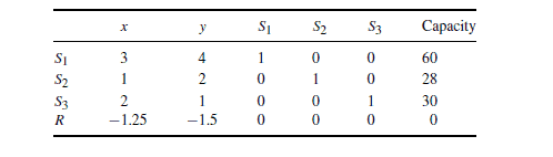
The first thing we want to do, in preparation for an algebraic technique, is to replace the system
of inequalities that describe the feasible set into a system of equations. But we already know
how to do that – we must include the slack variables $S_{1}, S_{2}$, and $S_{3} .$ Recall from Chapter 3 that
these represent the leftover resources of lemons, limes, and tablespoons of sugar, respectively. For
each resource, if you add the leftovers to what you’ve used up the result is the total amount of that
resource available. Thus, for example, the amount of lemons used is $3 x+4 y$, and $S_{1}$ is the number
$$ \begin{array}{l}3 x+4 y+S_{1}=60 . \ \text { of leftover lemons; therefore, the first inequality becomes } \ \text { Repeating the process for each structural constraint leads us to the following system of equa- } \ \text { tions: } \ \qquad \begin{aligned} 3 x+4 y+S_{1} &=60 \ x+2 y+S_{2} &=28 \ 2 x+y+S_{3} &=30 . \end{aligned}\end{array} $$
Of course, we must have $x \geq 0, y \geq 0$, and $S_{i} \geq 0$ for $i=1,2,3$ as well in order to obtain a feasible solution. We know from Chapter 1 that we can view a system of equations in three ways. into the simplex algorithm, but there is also the vector point of view. If we write the preceding system of equations as a vector equation, the result is We hope that the reader recognizes this equation – it is precisely Eq. (5.1) for this problem: In this way, since the simplex algorithm involves pivoting the system, which is equivalent to this vector equation, we may view the simplex algorithm as a natural algebraic extension of the method of graphing in the constraint space. Indeed, by Proposition $3.2$, we know the optimal point is a basic, feasible solution. The method of graphing in the constraint space was a brute force approach, where every basic, feasible solution was checked (in the case when $m=2$ ). The simplex algorithm is a way to generalize this to the case $m>2$, together with the improvement that we need not check every basic, feasible solution of Eq. (5.1) – we can usually arrive at the optimal solution after checking just a few of them. Now that we know the connection with the vector equation and the method of graphing in the constraint space, we will return to the point of view of writing the system of equations by using the augmented coefficient matrix, and base the simplex algorithm on pivoting this matrix. In order to motivate the steps of the pivoting process, it will be instructive to refer to the graph of the feasible set (in the decision space, of course, since this is two-dimensional) in Figure $4.1$. For connparison purposes, we also modify Table $3.3$ in Table $5.1$, where the coordinates of each corner were listed, along with the value of the objective function there, and we have added two Colunากns.

凸优化代考

在这一点上，我们可以只介绍第二阶段旋转的规则，读者可以通过死记硬背来学习它们。由于您已经从第 1 章熟悉了旋转，因此学习单纯形算法并不难。但是，我们想为这些规则提供一些动机，并解释算法背后的一些推理。所以，相反，我们将采取更好的方法来激励算法，而不是从熟悉的标准形式最大化问题开始？所以让问题：
5.1 标准形式最大化问题
187
为了准备代数技术，我们要做的第一件事是替换系统
将可行集描述为方程组的不等式。但我们已经知道
如何做到这一点 – 我们必须包括松弛变量 $S_{1}、S_{2}$ 和 $S_{3}。$ 回忆第 3 章
这些分别代表柠檬、酸橙和汤匙糖的剩余资源。为了
每个资源，如果你把剩下的加到你用完的东西上，结果就是那个总量
可用资源。因此，例如，柠檬的使用量是 $3 x+4 y$，$S_{1}$ 是数量
$$ \begin{array}{l}3 x+4 y+S_{1}=60 。 \ \text { 剩下的柠檬；因此，第一个不等式变为 } \ \text { 对每个结构约束重复该过程导致我们得到以下等式系统 } \ \text { tions: } \ \qquad \begin{aligned} 3 x+4 y+S_{1} &=60 \ x+2 y+S_{2} &=28 \ 2 x+y+S_{3} &=30 。 \end{对齐}\end{数组} $$
当然，我们必须有$x \geq 0, y \geq 0$ 和$S_{i} \geq 0$ for $i=1,2,3$ 以获得可行的解决方案。从第 1 章我们知道，我们可以用三种方式查看方程组。进入单纯形算法，但也有向量的观点。如果我们把前面的方程组写成向量方程，结果是我们希望读者能认出这个方程——它正是方程。 (5.1) 对于这个问题：这样，由于单纯形算法涉及到系统的旋转，这相当于这个向量方程，我们可以将单纯形算法看作是约束空间中绘图方法的自然代数扩展。事实上，根据命题 $3.2$，我们知道最优点是一个基本的、可行的解决方案。在约束空间中绘制图形的方法是一种蛮力方法，其中检查了每个基本可行的解决方案（在 $m=2$ 的情况下）。单纯形算法是一种将其推广到 $m>2$ 情况的方法，以及我们不需要检查方程的每个基本可行解的改进。 (5.1) – 我们通常可以在检查其中几个后得出最佳解决方案。现在我们知道了与向量方程的联系以及在约束空间中作图的方法，我们将回到使用增广系数矩阵编写方程组的观点，并将单纯形算法基于对这个矩阵进行旋转.为了激发旋转过程的步骤，参考图 $4.1$ 中的可行集图（当然，在决策空间中，因为这是二维的）将是有益的。出于对比目的，我们还修改了表 $5.1$ 中的表 $3.3$，其中列出了每个角的坐标以及目标函数的值，并且我们添加了两个 Colunากns。