数学代写| The Erd}os{Kac Theorem 数论代考
数论代考
We begin by recalling the statement (see Theorem 1.1.1), in its probabilistic phrasing:
THEOREM 2.3.1 (Erdős-Kac Theorem). For $\mathrm{N} \geqslant 1$, let $\Omega_{\mathrm{N}}={1, \ldots, \mathrm{N}}$ with the uniform probability measure $\mathbf{P}{\mathrm{N}}$. Let $\mathrm{X}{\mathrm{N}}$ be the random variable
$$
n \mapsto \frac{\omega(n)-\log \log \mathrm{N}}{\sqrt{\log \log \mathrm{N}}}
$$
on $\Omega_{\mathrm{N}}$ for $\mathrm{N} \geqslant 3$. Then $\left(\mathrm{X}{\mathrm{N}}\right){\mathrm{N} \geqslant 3}$ converges in law to a standard gaussian random variable, i.e., to a gaussian random variable with expectation 0 and variance 1 .
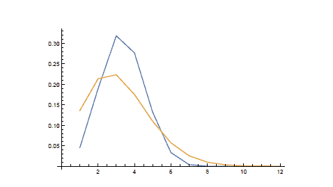
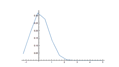
Figure $2.1$ shows a plot of the empirical density of $\mathrm{X}_{\mathrm{N}}$ for $\mathrm{N}=10^{10}$ : one can see something that could be the shape of the gaussian density appearing, but the fit is very far from perfect (we will comment later why this could be expected).
The original proof of Theorem $2.3 .1$ is due to Erdős and Kac in 1939 [35]. We will explain a proof following the work of Granville and Soundararajan [51] and of Billingsley $[9$, p. 394]. As usual, the presentation emphasizes the probabilistic nature of the argument.
As before, we begin by explaining why the statement can be considered to be unsurprising. This is an elaboration of the type of heuristic argument that we used to justify the limit in Theorem 2.2.1.
The arithmetic function $\omega$ is additive. Write
$$
\omega(n)=\sum_{p} \mathrm{~B}{p}(n) $$ for $n \in \Omega{\mathrm{N}}$, where $\mathrm{B}{p}$ is as usual the Bernoulli random variable on $\Omega{\mathrm{N}}$ that is the characteristic function of the event $p \mid n$. Using Proposition 1.3.7, the natural probabilistic guess for a limit (if there was one) would be the series
$$
\sum_{p} \mathrm{~B}{p} $$ where $\left(\mathrm{B}{p}\right)$ are independent Bernoulli random variables, as in Proposition 1.4.1. But this series diverges almost surely: indeed, the series
$$
\sum_{p} \mathrm{E}\left(\mathrm{B}{p}\right)=\sum{p} \frac{1}{p}
$$
diverges by the basic Mertens estimate from prime number theory, namely
$$
\sum_{p \leqslant \mathrm{~N}} \frac{1}{p}=\log \log \mathrm{N}+\mathrm{O}(1)
$$
for $\mathrm{N} \geqslant 3$ (see Proposition C.3.1 in Appendix C), so that the divergence follows from Kolmogorov’s Theorem B.10.1 (or indeed an application of the Borel-Cantelli Lemma, see Exercise B.10.4).
One can however refine the formula for $\omega$ by observing that $n \in \Omega_{\mathrm{N}}$ has no prime divisor larger than $\mathrm{N}$, so that we also have
$\frac{1}{p}=\log \log$ in Appendia indeed an la for $\omega$
$\omega(2.5)=\sum_{p \leqslant \mathrm{~N}} \mathrm{~B}{p}(n)$ for $n \in \Omega{N}$. Correspondingly, we may expect that the probabilistic distribution of $\omega$ on $\Omega_{\mathrm{N}}$ will be similar to that of the sum
$$
\sum_{p \leqslant \mathrm{~N}} \mathrm{~B}{p} $$ But the latter is a sum of independent (though not identically distributed) random variables, and its asymptotic behavior is therefore well-understood. In fact, a simple case of the Central Limit Theorem (see Theorem B.7.2) implies that the renormalized random variables $$ \frac{\sum{p \leqslant \mathrm{~N}} \mathrm{~B}{p}-\sum{p \leqslant \mathrm{~N}} p^{-1}}{\sqrt{\sum_{p \leqslant \mathrm{~N}} p^{-1}\left(1-p^{-1}\right)}}
$$
converge in law to a standard gaussian random variable. It is then to be expected that the arithmetic sums (2.5) are sufficiently close to (2.6) so that a similar renormalization of $\omega$ on $\Omega_{\mathrm{N}}$ will lead to the same limit, and this is exactly the statement of Theorem 2.3.1 (by the Mertens Formula again).
We now begin the rigorous proof. We will prove convergence in law using the method of moments, as explained in Section B.3 of Appendix B, specifically in Theorem B.5.5 and Remark B.5.9. This is definitely not the only way to confirm the heuristic above,
我们首先回顾一下概率性措辞中的陈述(参见定理 1.1.1):
定理 2.3.1(Erdős-Kac 定理)。对于 $\mathrm{N} \geqslant 1$,让 $\Omega_{\mathrm{N}}={1, \ldots, \mathrm{N}}$ 具有统一概率测度 $\mathbf{P} {\mathrm{N}}$。令 $\mathrm{X}{\mathrm{N}}$ 为随机变量
$$
n \mapsto \frac{\omega(n)-\log \log \mathrm{N}}{\sqrt{\log \log \mathrm{N}}}
$$
在 $\Omega_{\mathrm{N}}$ 上为 $\mathrm{N} \geqslant 3$。那么 $\left(\mathrm{X}{\mathrm{N}}\right){\mathrm{N} \geqslant 3}$ 收敛于一个标准的高斯随机变量,即一个高斯随机变量期望 0 和方差 1 。
图 $2.1$ 显示了 $\mathrm{X}_{\mathrm{N}}$ 对于 $\mathrm{N}=10^{10}$ 的经验密度图:可以看到可能是形状的东西高斯密度的出现,但拟合远非完美(我们稍后会评论为什么会出现这种情况)。
定理 $2.3 .1$ 的原始证明应归功于 Erdős 和 Kac 在 1939 年 [35]。我们将根据 Granville 和 Soundararajan [51] 以及 Billingsley $[9$, p. 394]。像往常一样,演示文稿强调了论点的概率性质。
和以前一样,我们首先解释为什么该陈述可以被认为是不足为奇的。这是我们用来证明定理 2.2.1 中的极限的启发式论证类型的详细说明。
算术函数$\omega$ 是加法的。写
$$
\omega(n)=\sum_{p} \mathrm{~B}{p}(n) $$ 对于 $n \in \Omega{\mathrm{N}}$,其中 $\mathrm{B}{p}$ 和往常一样是 $\Omega{\mathrm{N}}$ 上的伯努利随机变量,即事件 $p \mid n$ 的特征函数。使用命题 1.3.7,极限(如果有的话)的自然概率猜测将是系列
$$
\sum_{p} \mathrm{~B}{p} $$ 其中 $\left(\mathrm{B}{p}\right)$ 是独立的伯努利随机变量,如命题 1.4.1 所示。但是这个系列几乎肯定会发散:确实,系列
$$
\sum_{p} \mathrm{E}\left(\mathrm{B}{p}\right)=\sum{p} \frac{1}{p}
$$
与素数理论的基本 Mertens 估计不同,即
$$
\sum_{p \leqslant \mathrm{~N}} \frac{1}{p}=\log \log \mathrm{N}+\mathrm{O}(1)
$$
对于 $\mathrm{N} \geqslant 3$(参见附录 C 中的命题 C.3.1),因此分歧来自 Kolmogorov 定理 B.10.1(或者实际上是 Borel-Cantelli 引理的应用,参见练习 B.10.4 )。
然而,我们可以通过观察 $n \in \Omega_{\mathrm{N}}$ 没有大于 $\mathrm{N}$ 的素因数来改进 $\omega$ 的公式,因此我们也有
附录中的 $\frac{1}{p}=\log \log$ 确实是 $\omega$
$\omega(2.5)=\sum_{p \leqslant \mathrm{~N}} \mathrm{~B}{p}(n)$ 对于 $n \in \Omega{N}$。相应地,我们可以预期 $\omega$ 在 $\Omega_{\mathrm{N}}$ 上的概率分布将类似于 sum 的概率分布
$$
\sum_{p \leqslant \mathrm{~N}} \mathrm{~B}{p} $$ 但后者是独立(虽然不是同分布)随机变量的总和,因此它的渐近行为是众所周知的。事实上,中心极限定理(见定理 B.7.2)的一个简单例子意味着重整化随机变量 $$ \frac{\sum{p \leqslant \mathrm{~N}} \mathrm{~B}{p}-\sum{p \leqslant \mathrm{~N}} p^{-1}}{\sqrt {\sum_{p \leqslant \mathrm{~N}} p^{-1}\left(1-p^{-1}\right)}}
$$
收敛到一个标准的高斯随机变量。然后可以预期算术和 (2.5) 足够接近 (2.6),因此在 $\Omega_{\mathrm{N}}$ 上的 $\omega$ 的类似重整化将导致相同的限制,并且这正是定理 2.3.1 的陈述(再次由默滕斯公式)。
我们现在开始严格的证明。正如附录 B 的 B.3 节,特别是定理 B.5.5 和备注 B.5.9 中所解释的,我们将使用矩量法证明法律上的收敛性。这绝对不是确认上述启发式的唯一方法,
我们将命题 B.4.4 应用于随机向量 $\mathrm{G}{\mathrm{N}}=\left(g^{b}\left(\mathrm{~S}{\mathrm{N} }\right), g^{\sharp}\left(\mathrm{S}{\mathrm{N}}\right)\right)$(值在 $\mathrm{C}^{2}$ 中) , 有近似值 $\mathrm{G}{\mathrm{N}}=\mathrm{G}{\mathrm{N}, \mathrm{M}}+\mathrm{E}{\mathrm{N }, \mathrm{M}}$ 其中
$$
\mathrm{G}{\mathrm{N}, \mathrm{M}}=\left(\sum{p \leqslant \mathrm{M}} g^{b}\left(p^{v_{p} \left(\mathrm{~S}{\mathrm{N}}\right)}\right), \sum{p \leqslant \mathrm{M}} g^{\sharp}\left(p^{v_ {p}\left(\mathrm{~S}{\mathrm{N}}\right)}\right)\right) 。 $$ 让 $M \geqslant 1$ 固定。随机向量 $G{N, M}$ 是有限和,并且表示为 $\Omega_{\mathrm{N}}$ 的元素的估值 $v_{p}$ 的明显连续函数,对于 $p \leqslant \mathrm{M}$。由于这些估值的向量根据推论 1.3.9 在法律上收敛到 $\left(\mathrm{V}{p}\right){p \leqslant \mathrm{M}}$,因此应用连续映射的合成(同样是命题 B.3.2),因此 $\left(\mathrm{G}{\mathrm{N}, \mathrm{M}}\right){\mathrm{N}}$ 在规律上收敛为$\mathrm{N} \rightarrow+\infty$ 到向量
$$
\left(\sum_{p \leqslant \mathrm{M}} g^{b}\left(p^{\mathrm{V}{p}}\right), \sum{p \leqslant \mathrm{M }} g^{\sharp}\left(p^{\mathrm{V}_{p}}\right)\right) \text {. }
$$
因此,足以验证命题 B.4.4 的假设 (2) 成立,我们可以对向量的两个坐标中的每一个分别进行验证(通过对 $\mathrm{C}^{2}$ 取范数)在命题中是两个坐标的模的最大值)。
数论代写
数论是纯粹数学的分支之一,主要研究整数的性质。整数可以是方程式的解(丢番图方程)。有些解析函数(像黎曼ζ函数)中包括了一些整数、质数的性质,透过这些函数也可以了解一些数论的问题。透过数论也可以建立实数和有理数之间的关系,并且用有理数来逼近实数(丢番图逼近)。
按研究方法来看,数论大致可分为初等数论和高等数论。初等数论是用初等方法研究的数论,它的研究方法本质上说,就是利用整数环的整除性质,主要包括整除理论、同余理论、连分数理论。高等数论则包括了更为深刻的数学研究工具。它大致包括代数数论、解析数论、计算数论等等。

其他相关科目课程代写:组合学Combinatorics集合论Set Theory概率论Probability组合生物学Combinatorial Biology组合化学Combinatorial Chemistry组合数据分析Combinatorial Data Analysis
my-assignmentexpert愿做同学们坚强的后盾,助同学们顺利完成学业,同学们如果在学业上遇到任何问题,请联系my-assignmentexpert™,我们随时为您服务!
在中世纪时,除了1175年至1200年住在北非和君士坦丁堡的斐波那契有关等差数列的研究外,西欧在数论上没有什么进展。
数论中期主要指15-16世纪到19世纪,是由费马、梅森、欧拉、高斯、勒让德、黎曼、希尔伯特等人发展的。最早的发展是在文艺复兴的末期,对于古希腊著作的重新研究。主要的成因是因为丢番图的《算术》(Arithmetica)一书的校正及翻译为拉丁文,早在1575年Xylander曾试图翻译,但不成功,后来才由Bachet在1621年翻译完成。
计量经济学代考
计量经济学是以一定的经济理论和统计资料为基础,运用数学、统计学方法与电脑技术,以建立经济计量模型为主要手段,定量分析研究具有随机性特性的经济变量关系的一门经济学学科。 主要内容包括理论计量经济学和应用经济计量学。 理论经济计量学主要研究如何运用、改造和发展数理统计的方法,使之成为经济关系测定的特殊方法。
相对论代考
相对论(英語:Theory of relativity)是关于时空和引力的理论,主要由愛因斯坦创立,依其研究对象的不同可分为狭义相对论和广义相对论。 相对论和量子力学的提出给物理学带来了革命性的变化,它们共同奠定了现代物理学的基础。
编码理论代写
编码理论(英语:Coding theory)是研究编码的性质以及它们在具体应用中的性能的理论。编码用于数据压缩、加密、纠错,最近也用于网络编码中。不同学科(如信息论、电机工程学、数学、语言学以及计算机科学)都研究编码是为了设计出高效、可靠的数据传输方法。这通常需要去除冗余并校正(或检测)数据传输中的错误。
编码共分四类:[1]
数据压缩和前向错误更正可以一起考虑。
复分析代考
学习易分析也已经很冬年了,七七八人的也续了圧少的书籍和论文。略作总结工作,方便后来人学 Đ参考。
复分析是一门历史悠久的学科,主要是研究解析函数,亚纯函数在复球面的性质。下面一昭这 些基本内容。
(1) 提到复变函数 ,首先需要了解复数的基本性左和四则运算规则。怎么样计算复数的平方根, 极坐标与 $x y$ 坐标的转换,复数的模之类的。这些在高中的时候囸本上都会学过。
(2) 复变函数自然是在复平面上来研究问题,此时数学分析里面的求导数之尖的运算就会很自然的 引入到复平面里面,从而引出解析函数的定义。那/研究解析函数的性贡就是关楗所在。最关键的 地方就是所谓的Cauchy一Riemann公式,这个是判断一个函数是否是解析函数的关键所在。
(3) 明白解析函数的定义以及性质之后,就会把数学分析里面的曲线积分 $a$ 的概念引入复分析中, 定义几乎是一致的。在引入了闭曲线和曲线积分之后,就会有出现复分析中的重要的定理: Cauchy 积分公式。 这个是易分析的第一个重要定理。