运筹学(Operation)是近代应用数学的一个分支。它把具体的问题进行数学抽象,然后用像是统计学、数学模型和算法等方法加以解决,以此来寻找复杂问题中的最佳或近似最佳的解答。
作为专业的留学生服务机构,Assignmentexpert™多年来已为美国、英国、加拿大、澳洲等留学热门地的学生提供专业的学术服务,包括但不限于论文代写,A作业代写,Dissertation代写,Report代写,Paper代写,Presentation代写,网课代修等等。为涵盖高中,本科,研究生等海外留学生提供辅导服务,辅导学科包括数学,物理,统计,化学,金融,经济学,会计学等全球99%专业科目。写作团队既有专业英语母语作者,也有海外名校硕博留学生,每位写作老师都拥有过硬的语言能力,专业的学科背景和学术写作经验。我们承诺100%原创,100%专业,100%准时,100%满意。
my-assignmentexpert愿做同学们坚强的后盾,助同学们顺利完成学业,同学们如果在学业上遇到任何问题,请联系my-assignmentexpert™,我们随时为您服务!
运筹学代写
The concept underlying interior-point methods for linear programming is to use nonlinear programming techniques of analysis and methodology. The analysis is often based on differentiation of the functions defining the problem. Traditional linear programming does not require these techniques since the defining functions are linear. Duality in general nonlinear programs is typically manifested through Lagrange multipliers (which are called dual variables in linear programming). The analysis and algorithms of the remaining sections of the chapter use these nonlinear techniques. These techniques are discussed systematically in later chapters, so rather detail in their application to linear programming. It is expected that most readers are already familiar with the basic method for minimizing a function by setting its derivative to zero, and for incorporating constraints by introducing Lagrange multipliers. These methods are discussed in detail in Chaps. 11-15.
The computational algorithms of nonlinear programming are typically iterative in nature, often characterized as search algorithms. At any step with a given point, a direction for search is established and then a move in that direction is made to are systematically presented throughout the text. In this chapter, we use versions of Newton’s method as the search algorithm, but we postpone a detailed study of the method until later chapters.
(5.5) Not only have nonlinear methods improved linear programming, but interiorpoint methods for linear programming have been extended to provide new approaches to nonlinear programming. This chapter is intended to show how this merger of linear and nonlinear programming produces elegant and effective programming. Study of them here, even without all the detailed analysis, should provide good intuitive background for the more general manifestations. Consider a primal linear program in standard form
$\begin{aligned} \text { (LP) } \operatorname{minimize} & \mathbf{c}^{T} \mathbf{x} \ \text { subject to } & \mathbf{A x}=\mathbf{b}, \mathbf{x} \geqslant \mathbf{0} . \end{aligned}$
We denote the feasible region of this program by $\mathcal{F}{p}$. We assume that $\dot{\mathcal{F}}{p}={\mathbf{x}$ : $\mathbf{A x}=\mathbf{b}, \mathbf{x}>\mathbf{0}}$ is nonempty and the optimal solution set of the problem is bounded. Associated with this problem, we define for $\mu \geqslant 0$ the barrier problem
$$
\begin{aligned}
&\text { (BP) minimize } \mathbf{c}^{T} \mathbf{x}-\mu \sum_{j=1}^{n} \log x_{j} \
&\text { subject to } \mathbf{A x}=\mathbf{b}, \mathbf{x}>\mathbf{0}
\end{aligned}
$$
5 Interior-Point Methods
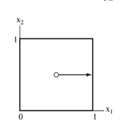
142 It is clear that $\mu=0$ corresponds to the original problem $(5.5)$. As $\mu \rightarrow \infty$, the solution approaches the analytic center of the feasible region (when it is bounded), since the barrier term swamps out $\mathbf{c}^{T} \mathbf{x}$ in the objective. As $\mu$ is varied continuously toward 0 , there is a path $\mathbf{x}(\mu)$ defined by the solution to (BP). This path $\mathbf{x}(\mu)$ is termed the primal central path. As $\mu \rightarrow 0$ this path converges to the analytic center of the op of (LP).
A strategy for solving (LP) is to solve (BP) for smaller and smaller values of $\mu$ and thereby approach a solution to (LP). This is indeed the basic idea of interior- point methods. point methods.
At any $\mu>0$, under the assumptions that we have made for problem (5.5), the necessary and sufficient conditions for a unique and bounded solution are obtained form the Lagrangian (see Chap. 11)
$$
\mathbf{c}^{T} \mathbf{x}-\mu \sum_{j=1}^{n} \log x_{j}-\mathbf{y}^{T}(\mathbf{A} \mathbf{x}-\mathbf{b})
$$
The derivatives with respect to the $x_{j}$ ‘s are set to zero, leading to the conditions
$$
c_{j}-\mu / x_{j}-\mathbf{y}^{T} \mathbf{a}{j}=0, \text { for each } j $$ form the Lagrangia The derivatives or equivalently where as before $\mathbf{a}{j}$ is the $j$ th column of $\mathbf{A}, \mathbf{1}$ is the vector of 1’s, and $\mathbf{X}$ is the diagonal matrix whose diagonal entries are the components of $\mathbf{x}>\mathbf{0}$. Setting $s_{j}=\mu / x_{j}$ the complete set of conditions can be rewritten
$$
\begin{aligned}
\mathbf{x} \circ \mathrm{s} &=\boldsymbol{\mu} \mathbf{1} \
\mathbf{A x} &=\mathbf{b}
\end{aligned}
$$
线性规划内点法的基本概念是使用非线性规划技术的分析和方法。分析通常基于定义问题的功能的区分。传统的线性规划不需要这些技术,因为定义函数是线性的。一般非线性程序中的对偶性通常通过拉格朗日乘数(在线性规划中称为对偶变量)表现出来。本章其余部分的分析和算法使用这些非线性技术。这些技术将在后面的章节中系统地讨论,因此更详细地介绍了它们在线性规划中的应用。预计大多数读者已经熟悉通过将函数的导数设置为零来最小化函数的基本方法,以及通过引入拉格朗日乘子来合并约束的基本方法。这些方法将在章节中详细讨论。 11-15。
非线性规划的计算算法本质上通常是迭代的,通常以搜索算法为特征。在给定点的任何步骤中,都会建立搜索方向,然后在该方向上进行移动以系统地呈现在整个文本中。在本章中,我们使用牛顿方法的版本作为搜索算法,但我们将对该方法的详细研究推迟到后面的章节。
(5.5) 非线性方法不仅改进了线性规划,而且线性规划的内点方法也得到了扩展,为非线性规划提供了新的方法。本章旨在展示线性和非线性编程的这种结合如何产生优雅而有效的编程。在这里对它们进行研究,即使没有所有详细的分析,也应该为更普遍的表现提供良好的直观背景。考虑标准形式的原始线性程序
$\begin{aligned} \text { (LP) } \operatorname{minimize} & \mathbf{c}^{T} \mathbf{x} \ \text { 服从 } & \mathbf{A x}=\ mathbf{b}, \mathbf{x} \geqslant \mathbf{0} 。 \end{对齐}$
我们用 $\mathcal{F}{p}$ 表示这个程序的可行域。我们假设 $\dot{\mathcal{F}}{p}={\mathbf{x}$ : $\mathbf{A x}=\mathbf{b}, \mathbf{x}>\mathbf{ 0}}$ 是非空的,问题的最优解集是有界的。与这个问题相关,我们为 $\mu \geqslant 0$ 定义了障碍问题
$$
\开始{对齐}
&\text { (BP) 最小化 } \mathbf{c}^{T} \mathbf{x}-\mu \sum_{j=1}^{n} \log x_{j} \
&\text { 服从 } \mathbf{A x}=\mathbf{b}, \mathbf{x}>\mathbf{0}
\end{对齐}
$$
5 内点法
142 很明显,$\mu=0$ 对应于原始问题 $(5.5)$。由于 $\mu \rightarrow \infty$,解接近可行域的解析中心(当它有界时),因为障碍项淹没了 $\mathbf{c}^{T} \mathbf{x}$目标。由于 $\mu$ 不断地向 0 变化,因此 (BP) 的解定义了一条路径 $\mathbf{x}(\mu)$。这条路径 $\mathbf{x}(\mu)$ 被称为原始中心路径。由于 $\mu \rightarrow 0$,这条路径收敛到 (LP) 的运算的解析中心。
求解 (LP) 的策略是求解 (BP) 以获得越来越小的 $\mu$ 值,从而逼近 (LP) 的解。这确实是内点方法的基本思想。点方法。
在任何 $\mu>0$ 处,在我们对问题 (5.5) 所做的假设下,从拉格朗日算子可以得到唯一且有界解的充分必要条件(见第 11 章)
$$
\mathbf{c}^{T} \mathbf{x}-\mu \sum_{j=1}^{n} \log x_{j}-\mathbf{y}^{T}(\mathbf{A} \mathbf{x}-\mathbf{b})
$$
关于 $x_{j}$ 的导数设置为零,导致条件
$$
c_{j}-\mu / x_{j}-\mathbf{y}^{T} \mathbf{a}{j}=0, \text { for each } j $$ 形成 Lagrangia 导数或等价物 其中 $\mathbf{a}{j}$ 是 $\mathbf{A} 的第 $j$ 列,\mathbf{1}$ 是 1 的向量,$\mathbf{X}$ 是对角矩阵,其对角元素是 $\mathbf{x}>\mathbf{0}$ 的分量。设置 $s_{j}=\mu / x_{j}$ 可以重写完整的条件集
$$
\开始{对齐}
\mathbf{x} \circ \mathrm{s} &=\boldsymbol{\mu} \mathbf{1} \
\mathbf{A x} &=\mathbf{b}
\end{对齐}
$$
运筹学代考

什么是运筹学代写
运筹学(OR)是一种解决问题和决策的分析方法,在组织管理中很有用。在运筹学中,问题被分解为基本组成部分,然后通过数学分析按定义的步骤解决。
运筹学的过程大致可以分为以下几个步骤:
- 确定需要解决的问题。
- 围绕问题构建一个类似于现实世界和变量的模型。
- 使用模型得出问题的解决方案。
- 在模型上测试每个解决方案并分析其成功。
- 实施解决实际问题的方法。
与运筹学交叉的学科包括统计分析、管理科学、博弈论、优化理论、人工智能和复杂网络分析。所有这些学科的目标都是解决某一个现实中出现的复杂问题或者用数学的方法为决策提供指导。 运筹学的概念是在二战期间由参与战争的数学家们提出的。二战后,他们意识到在运筹学中使用的技术也可以被应用于解决商业、政府和社会中的问题。
运筹学代写的三个特点
所有运筹学解决实际问题的过程中都具有三个主要特征:
- 优化——运筹学的目的是在给定的条件下达到某一机器或者模型的最佳性能。优化还涉及比较不同选项和缩小潜在最佳选项的范围。
- 模拟—— 这涉及构建模型,以便在应用解决方案刀具体的复杂大规模问题之前之前尝试和测试简单模型的解决方案。
- 概率和统计——这包括使用数学算法和数据挖掘来发现有用的信息和潜在的风险,做出有效的预测并测试可能的解决方法。
运筹学领域提供了比普通软件和数据分析工具更强大的决策方法。此外,运筹学可以根据特定的业务流程或用例进行定制,以确定哪些技术最适合解决问题。
运筹学可以应用于各种活动,比如:计划和时间管理(Planning and Time Management),城乡规划(Urban and Rural Planning),企业资源计划(ERP)与供应链管理(Supply Chain Management)等等。 如有代写代考需求,欢迎同学们联系Assignmentexpert™,我们期待为你服务!