如果你也在 怎样金融数学Financial Mathematics这个学科遇到相关的难题,请随时右上角联系我们的24/7代写客服。金融数学Financial Mathematics是将数学方法应用于金融问题。(有时使用的同等名称是定量金融、金融工程、数学金融和计算金融)。它借鉴了概率、统计、随机过程和经济理论的工具。传统上,投资银行、商业银行、对冲基金、保险公司、公司财务部和监管机构将金融数学的方法应用于诸如衍生证券估值、投资组合结构、风险管理和情景模拟等问题。依赖商品的行业(如能源、制造业)也使用金融数学。 定量分析为金融市场和投资过程带来了效率和严谨性,在监管方面也变得越来越重要。
定量金融作为经济学的一个子领域,关注资产和金融工具的估值以及资源的配置。几个世纪的经验产生了关于经济运行方式和我们评估资产的方式的基本理论。模型描述了基本变量之间的关系,如资产价格、市场运动和利率。这些数学工具使我们能够得出原本难以发现或从直觉上无法立即看出的结论。模型应用的一个例子是银行的压力测试。 特别是在现代计算技术的帮助下,我们可以存储大量的数据并同时对许多变量进行建模,从而有能力对相当大和复杂的系统进行建模。因此,科学计算的技术,如数值分析、蒙特卡洛模拟和优化是金融数学的重要组成部分。
任何科学的很大一部分都是在对研究对象的基本了解的基础上建立可检验的假设,并通过可重复的研究来证明或反驳这些假设的能力。从这个角度来看,数学是代表理论的语言,并提供测试其有效性的工具。例如,在布莱克、斯科尔斯和默顿的期权定价理论中,提出了一个股票价格变动的模型,结合无风险投资将获得无风险收益率的理论,研究者们推断出可以给期权分配一个价值。
my-assignmentexpert™金融数学Financial Mathematics作业代写,免费提交作业要求, 满意后付款,成绩80\%以下全额退款,安全省心无顾虑。专业硕 博写手团队,所有订单可靠准时,保证 100% 原创。my-assignmentexpert™, 最高质量的金融数学Financial Mathematics作业代写,服务覆盖北美、欧洲、澳洲等 国家。 在代写价格方面,考虑到同学们的经济条件,在保障代写质量的前提下,我们为客户提供最合理的价格。 由于统计Statistics作业种类很多,同时其中的大部分作业在字数上都没有具体要求,因此金融数学Financial Mathematics作业代写的价格不固定。通常在经济学专家查看完作业要求之后会给出报价。作业难度和截止日期对价格也有很大的影响。
想知道您作业确定的价格吗? 免费下单以相关学科的专家能了解具体的要求之后在1-3个小时就提出价格。专家的 报价比上列的价格能便宜好几倍。
my-assignmentexpert™ 为您的留学生涯保驾护航 在金融数学Financial Mathematics作业代写方面已经树立了自己的口碑, 保证靠谱, 高质且原创的金融数学Financial Mathematics代写服务。我们的专家在金融数学Financial Mathematics代写方面经验极为丰富,各种金融数学Financial Mathematics相关的作业也就用不着 说。
我们提供的金融数学Financial Mathematics及其相关学科的代写,服务范围广, 其中包括但不限于:
- 随机微积分 Stochastic calculus
- 随机分析 Stochastic analysis
- 随机控制理论 Stochastic control theory
- 微观经济学 Microeconomics
- 数量经济学 Quantitative Economics
- 宏观经济学 Macroeconomics
- 经济统计学 Economic Statistics
- 经济学理论 Economic Theory
- 计量经济学 Econometrics
经济代写
数学代写|金融数学作业代写Financial Mathematics代考|Applications
Modeling dynamics of asset prices plays important role in a lot of microeconomics problems. For example, by understanding the behavior of stock prices, one can take good decision for a portfolio. Continuous-time random walk process is a suitable class of process for modeling the behavior of high frequency data.
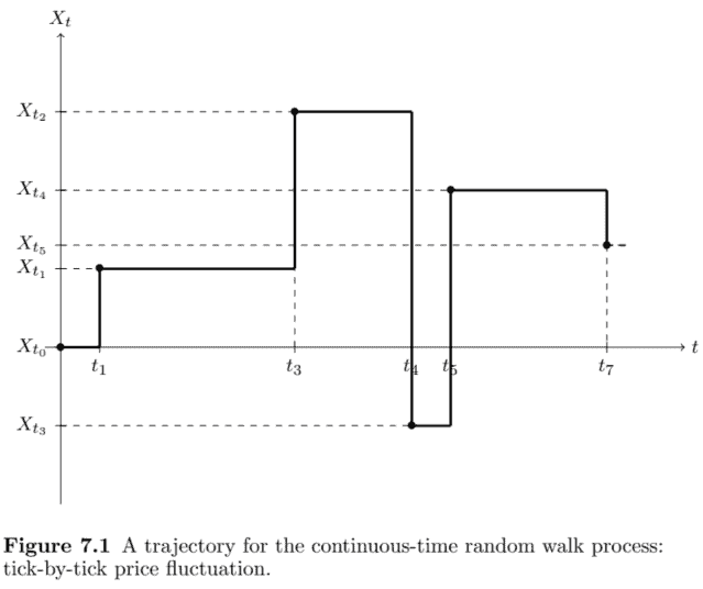
Figure $7.1$ shows a trajectory for the continuous-time random walk. It shows two random variables play important role in the structure of this process: jump magnitude, and waiting time. Unlike the random walk, the waiting time for jumps is not the same during time. It is perfect to describe the behavior of dynamics of high frequency market. More precisely, since the business activity for all trading periods are not the same. ${ }^{8}$ Some days we have more activity and some days less. The waiting time random variable describes this property.
In the continuous-time random walk setting the calender time, $t$, is replaced with business time, waiting time random variable. Clark (1973) for the first time tried to recover normality assumption of distribution for the time series of return process. His ideas are applied to the option pricing with pure jump Lévy process. These pure jump Lévy process can be obtained by changing the time of a Brownian motion with a subordinator. Variance-gamma, normal inverse Gaussian, and CGMY process are pure jump Lévy process that can be obtained by changing time of Brownian motion with a subordinator. ${ }^{9}$
数学代写|金融数学作业代写 Financial Mathematics代考|DYNAMICS OF THE ASSET PRICES
The initial setting for implementing the continuous-time random walk for studying the behavior of asset prices is as follows. Denote the waiting times between each trade by $\left{j_{1}, j_{2}, \cdots, j_{n}, \cdots\right}$. Let $\left(P_{t}\right){t \geq 0}$ and $S{t}=\log \left(P_{t}\right)$ be the price process and log-price of an asset at time $t$. The waiting time random variables are independent and identically distributed. Let $X_{1}, X_{2}, \cdots, X_{n}, \cdots$ be the log-return process, more specifically, $X_{n}$ is given by
$$
X_{n}=S_{n}-S_{n-1}=\log \left(P_{n}\right)-\log \left(P_{n-1}\right)=\log \left(\frac{P_{n}}{P_{n-1}}\right)
$$
Without loss of generality we assume $X_{0}=0$. Bear in mind that the log-return is more convenient to study the behavior of asset price. ${ }^{10}$ Moreover, the log-return random variables are independent and identically distributed.
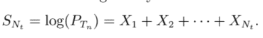
As explained earlier, the continuous-time random walk process is classified into two cases: uncoupled and coupled. If the random variables $j_{n}$ and $\Delta X_{n}$ are independent for each value of $n$, then $X_{n}$ is called an uncoupled continuoustime random walk process, and if they are dependent, $X_{n}$ is called a coupled continuous-time random walk process. Let $T_{n}=j_{1}+j_{2}+\cdots+j_{n}$ be the time $n$th trade. The number of trades by time $t>0$ is $N_{t}=\max \left{n: T_{n} \leq t\right}$, and therefore, the log-price at time $t$ is given by
$$
S_{N_{t}}=\log \left(P_{T_{n}}\right)=X_{1}+X_{2}+\cdots+X_{N_{t}} .
$$
Equation (7.7) is a subordinated process. More specifically, the calender time, $t$, for the stochastic process $S_{t}$ is changed with business time, $N_{t}$. If the waiting times are exponentially distributed, the continuous-time random walk process is a compound Poisson process. Therefore, the continuous-time random process is a Markovian process that belongs to the class of Lévy processes. In this case, the distribution for the log-price is Gaussian and for the price the distribution is log-normal.
The asymptotic theory for the continuous-time random walk process provides a useful tool for the application of this process. In fact, in order to estimate the parameter of interest one should estimate parameters of asymptotic distributions. In the previous section we discussed an approach for obtaining the probability density function for a continuous-time random walk for both the coupled and uncoupled cases.
数学代写|金融数学作业代写FINANCIAL MATHEMATICS代考|APPLICATIONS
资产价格动态建模在许多微观经济学问题中发挥着重要作用。例如,通过了解股票价格的行为,可以为投资组合做出正确的决策。连续时间随机游走过程是一类适合对高频数据行为进行建模的过程。
数字7.1显示了连续时间随机游走的轨迹。它表明两个随机变量在这个过程的结构中起着重要作用:跳跃幅度和等待时间。与随机游走不同,跳跃的等待时间在时间上是不一样的。可以完美地描述高频市场的动态行为。更准确地说,因为所有交易期间的业务活动都不相同。8有时我们活动较多,有时活动较少。等待时间随机变量描述了这个属性。
在设置日历时间的连续时间随机游走中,吨, 换成营业时间,等待时间随机变量。克拉克1973首次尝试恢复回归过程时间序列分布的正态假设。他的想法被应用于纯跳跃 Lévy 过程的期权定价。这些纯跳跃 Lévy 过程可以通过用从属子改变布朗运动的时间来获得。Variance-gamma、Normal Inverse Gaussian 和 CGMY process 是纯跳跃 Lévy 过程,可以通过用从属子改变布朗运动的时间来获得。9
数学代写|金融数学作业代写 FINANCIAL MATHEMATICS代考|DYNAMICS OF THE ASSET PRICES
实施用于研究资产价格行为的连续时间随机游走的初始设置如下。表示每笔交易之间的等待时间
between each trade by $\left{j_{1}, j_{2}, \cdots, j_{n}, \cdots\right}$. Let $\left(P_{t}\right){t \geq 0}$ and $S{t}=\log \left(P_{t}\right)$ be the price process and log-price of an asset at time $t$. The waiting time random variables are independent and identically distributed. Let $X_{1}, X_{2}, \cdots, X_{n}, \cdots$ be the
log-return process, more specifically, $X_{n}$ is given by
$$
X_{n}=S_{n}-S_{n-1}=\log \left(P_{n}\right)-\log \left(P_{n-1}\right)=\log \left(\frac{P_{n}}{P_{n-1}}\right)
$$
此外,对数返回随机变量是独立同分布的。
如前所述,连续时间随机游走过程分为两种情况:非耦合和耦合。如果随机变量jn和ΔXn是独立的每个值n, 然后Xn被称为非耦合连续时间随机游走过程,如果它们是依赖的,Xn称为耦合连续时间随机游走过程。让吨n=j1+j2+⋯+jn是时候n贸易。按时间划分的交易数量吨>0是N_{t}=\max \left{n: T_{n} \leq t\right}N_{t}=\max \left{n: T_{n} \leq t\right},因此,时间的对数价格吨是(谁)给的
小号ñ吨=日志(磷吨n)=X1+X2+⋯+Xñ吨.
方程7.7是一个从属的过程。更具体地说,日历时间,吨, 对于随机过程小号吨随营业时间而改变,ñ吨. 如果等待时间呈指数分布,则连续时间随机游走过程是复合泊松过程。因此,连续时间随机过程是属于 Lévy 过程的马尔可夫过程。在这种情况下,对数价格的分布是高斯分布,而价格的分布是对数正态分布。
连续时间随机游走过程的渐近理论为该过程的应用提供了有用的工具。事实上,为了估计感兴趣的参数,我们应该估计渐近分布的参数。在上一节中,我们讨论了一种获取耦合和非耦合情况下连续时间随机游走概率密度函数的方法。

计量经济学代写请认准my-assignmentexpert™ Economics 经济学作业代写
微观经济学代写请认准my-assignmentexpert™ Economics 经济学作业代写
宏观经济学代写请认准my-assignmentexpert™ Economics 经济学作业代写