如果你也在 怎样金融数学Financial Mathematics这个学科遇到相关的难题,请随时右上角联系我们的24/7代写客服。金融数学Financial Mathematics是将数学方法应用于金融问题。(有时使用的同等名称是定量金融、金融工程、数学金融和计算金融)。它借鉴了概率、统计、随机过程和经济理论的工具。传统上,投资银行、商业银行、对冲基金、保险公司、公司财务部和监管机构将金融数学的方法应用于诸如衍生证券估值、投资组合结构、风险管理和情景模拟等问题。依赖商品的行业(如能源、制造业)也使用金融数学。 定量分析为金融市场和投资过程带来了效率和严谨性,在监管方面也变得越来越重要。
定量金融作为经济学的一个子领域,关注资产和金融工具的估值以及资源的配置。几个世纪的经验产生了关于经济运行方式和我们评估资产的方式的基本理论。模型描述了基本变量之间的关系,如资产价格、市场运动和利率。这些数学工具使我们能够得出原本难以发现或从直觉上无法立即看出的结论。模型应用的一个例子是银行的压力测试。 特别是在现代计算技术的帮助下,我们可以存储大量的数据并同时对许多变量进行建模,从而有能力对相当大和复杂的系统进行建模。因此,科学计算的技术,如数值分析、蒙特卡洛模拟和优化是金融数学的重要组成部分。
任何科学的很大一部分都是在对研究对象的基本了解的基础上建立可检验的假设,并通过可重复的研究来证明或反驳这些假设的能力。从这个角度来看,数学是代表理论的语言,并提供测试其有效性的工具。例如,在布莱克、斯科尔斯和默顿的期权定价理论中,提出了一个股票价格变动的模型,结合无风险投资将获得无风险收益率的理论,研究者们推断出可以给期权分配一个价值。
my-assignmentexpert™金融数学Financial Mathematics作业代写,免费提交作业要求, 满意后付款,成绩80\%以下全额退款,安全省心无顾虑。专业硕 博写手团队,所有订单可靠准时,保证 100% 原创。my-assignmentexpert™, 最高质量的金融数学Financial Mathematics作业代写,服务覆盖北美、欧洲、澳洲等 国家。 在代写价格方面,考虑到同学们的经济条件,在保障代写质量的前提下,我们为客户提供最合理的价格。 由于统计Statistics作业种类很多,同时其中的大部分作业在字数上都没有具体要求,因此金融数学Financial Mathematics作业代写的价格不固定。通常在经济学专家查看完作业要求之后会给出报价。作业难度和截止日期对价格也有很大的影响。
想知道您作业确定的价格吗? 免费下单以相关学科的专家能了解具体的要求之后在1-3个小时就提出价格。专家的 报价比上列的价格能便宜好几倍。
my-assignmentexpert™ 为您的留学生涯保驾护航 在金融数学Financial Mathematics作业代写方面已经树立了自己的口碑, 保证靠谱, 高质且原创的金融数学Financial Mathematics代写服务。我们的专家在金融数学Financial Mathematics代写方面经验极为丰富,各种金融数学Financial Mathematics相关的作业也就用不着 说。
我们提供的金融数学Financial Mathematics及其相关学科的代写,服务范围广, 其中包括但不限于:
- 随机微积分 Stochastic calculus
- 随机分析 Stochastic analysis
- 随机控制理论 Stochastic control theory
- 微观经济学 Microeconomics
- 数量经济学 Quantitative Economics
- 宏观经济学 Macroeconomics
- 经济统计学 Economic Statistics
- 经济学理论 Economic Theory
- 计量经济学 Econometrics
经济代写
数学代写|金融数学作业代写Financial Mathematics代考|Fractionally Integrated
Fractionally integrated time series was introduced operationally in Granger (1980), Granger and Joyeux (1980), and Hosking (1981). Let’s recall that an autoregressive moving-average model of integrated time series (ARIMA) is written as follows:
$$
a(L)(1-L) y_{t}=b(L) \varepsilon_{t}
$$
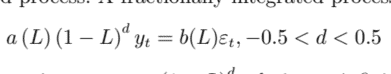
where $a(L), b(L)$ are polynomials in the lag operator $L$ and $\varepsilon_{t}$ is a zero-mean serially uncorrelated process. A fractionally integrated process is written as:
$$
a(L)(1-L)^{d} y_{t}=b(L) \varepsilon_{t},-0.5<d<0.5
$$
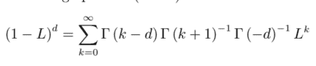
The fractional differencing operator $(1-L)^{d}$ admits an infinite expansion:
$$
(1-L)^{d}=\sum_{k=0}^{\infty} \Gamma(k-d) \Gamma(k+1)^{-1} \Gamma(-d)^{-1} L^{k}
$$
数学代写|金融数学作业代写 Financial Mathematics代考|stationary and invertible
For $-0.5<d<0.5$ the process $y_{t}$ is stationary and invertible and for $0<d<$ $0.5$ the process has long memory in the sense that the sum $\sum_{i=-k}^{k}\left|\rho_{i}\right|$, where $\rho_{i}$ is the autocorrelation at lag $i$ does not converge when $k$ tends to infinity.
The definition of fractional time series given above is based on an infinite moving average of noise terms. Johansen (2008) described a Vector Autoregressive Model whose solution is a fractionally integrated time series and which also allows for fractional cointegration. Granger (1986) had already suggested a notion of fractional cointegration, proposing the following model:
$$
a^{}(L)(1-L)^{d} y_{t}=\left(1-(1-L)^{d}\right)(1-L)^{d-b} \alpha \beta^{\prime} y_{t}+b(L) \epsilon_{t} $$ where $\epsilon_{t}$ is a sequence of i.i.d variables with positive definite covariance matrix. Johansen (2008) proposed a different VAR model. Lets define the “lag operator” $L_{d}=\left(1-(1-L)^{d}\right)$ which, as observed already in Granger (1986), plays a role similar to the lag operator. The model proposed in Johansen (2008) is written as: $$ A\left(L_{d}\right)(1-L)^{d} y_{t}=\left(1-(1-L)^{d}\right)(1-L)^{d-b} \alpha \beta^{\prime} y_{t}+b(L) \epsilon_{t} $$ In the Johansen (2008) model the polynomial $A$ is defined on the lag operator $L_{d}$ while in the Granger (1986) model the polynomial $a^{}$ was defined on the usual lag operator $L$.
数学代写|金融数学作业代写FINANCIAL MATHEMATICS代考|FRACTIONALLY INTEGRATED
在 Granger 中引入了分数积分时间序列1980,格兰杰和梅里1980, 和霍斯金1981. 让我们回顾一下集成时间序列的自回归移动平均模型一种R一世米一种写成如下:
一种(一世)(1−一世)和吨=b(一世)e吨
在哪里一种(一世),b(一世)是滞后算子中的多项式一世和e吨是一个零均值序列不相关过程。一个部分集成的过程写成:
一种(一世)(1−一世)d和吨=b(一世)e吨,−0.5<d<0.5
分数差分运算符(1−一世)d允许无限展开:
(1−一世)d=∑到=0∞Γ(到−d)Γ(到+1)−1Γ(−d)−1一世到
$$
A\left(L_{d}\right)(1-L)^{d} y_{t}=\left(1-(1-L)^{d}\right)(1-L)^{d-b} \alpha \beta^{\prime} y_{t}+b(L) \epsilon_{t}
$$
In the Johansen (2008) model the polynomial $A$ is defined on the lag operator $L_{d}$ while in the Granger (1986) model the polynomial $a^{*}$ was defined on the usual lag operator $L$.
The Johansen model is not a fractional ARIMA model which is defined as:
$$
D(L)(1-L)^{d} y_{t}=B(L) \epsilon_{t}
$$
数学代写|金融数学作业代写 FINANCIAL MATHEMATICS代考|STATIONARY AND INVERTIBLE
为了−0.5<d<0.5过程和吨是静止的和可逆的并且对于0<d< 0.5这个过程有很长的记忆,因为总和∑一世=−到到|ρ一世|, 在哪里ρ一世是滞后的自相关一世不收敛时到趋于无穷大。
上面给出的分数时间序列的定义是基于噪声项的无限移动平均值。约翰森2008描述了一个向量自回归模型,它的解决方案是分数积分时间序列,并且还允许分数协积分。格兰杰1986已经提出了分数协整的概念,提出了以下模型:

计量经济学代写请认准my-assignmentexpert™ Economics 经济学作业代写
微观经济学代写请认准my-assignmentexpert™ Economics 经济学作业代写
宏观经济学代写请认准my-assignmentexpert™ Economics 经济学作业代写