如果你也在 怎样代写微分方程differential equation这个学科遇到相关的难题,请随时右上角联系我们的24/7代写客服。微分方程differential equation在数学中,是将一个或多个未知函数及其导数联系起来的方程。在应用中,函数通常代表物理量,导数代表其变化率,而微分方程则定义了两者之间的关系。这种关系很常见;因此,微分方程在许多学科,包括工程、物理学、经济学和生物学中发挥着突出作用。
微分方程differential equation研究主要包括研究其解(满足每个方程的函数集合),以及研究其解的性质。只有最简单的微分方程可以用明确的公式求解;然而,一个给定的微分方程的解的许多属性可以在不精确计算的情况下确定。
my-assignmentexpert™ 微分方程differential equation作业代写,免费提交作业要求, 满意后付款,成绩80\%以下全额退款,安全省心无顾虑。专业硕 博写手团队,所有订单可靠准时,保证 100% 原创。my-assignmentexpert™, 最高质量的微分方程differential equation作业代写,服务覆盖北美、欧洲、澳洲等 国家。 在代写价格方面,考虑到同学们的经济条件,在保障代写质量的前提下,我们为客户提供最合理的价格。 由于统计Statistics作业种类很多,同时其中的大部分作业在字数上都没有具体要求,因此微分方程differential equation作业代写的价格不固定。通常在经济学专家查看完作业要求之后会给出报价。作业难度和截止日期对价格也有很大的影响。
想知道您作业确定的价格吗? 免费下单以相关学科的专家能了解具体的要求之后在1-3个小时就提出价格。专家的 报价比上列的价格能便宜好几倍。
my-assignmentexpert™ 为您的留学生涯保驾护航 在数学mathematics作业代写方面已经树立了自己的口碑, 保证靠谱, 高质且原创的微分方程differential equation代写服务。我们的专家在数学mathematics代写方面经验极为丰富,各种微分方程differential equation相关的作业也就用不着 说。
我们提供的微分方程differential equation及其相关学科的代写,服务范围广, 其中包括但不限于:
数学代写|微分方程代写differential equation代考|Mathematical forms of initial value problems
In this section, the first-order explicit differential equation format is presented, which can be regarded as the fundamental basis for numerical algorithms presented later.
Definition 3.1. The mathematical model of a first-order explicit differential equation is given by
$$
\boldsymbol{x}^{\prime}(t)=\boldsymbol{f}(t, \boldsymbol{x}(t))
$$
where the vector $\boldsymbol{x}(t)=\left[x_{1}(t), x_{2}(t), \ldots, x_{n}(t)\right]^{\mathrm{T}}$ is known as the state vector, and the function vector $\boldsymbol{f}(\cdot)=\left[f_{1}(\cdot), f_{2}(\cdot), \ldots, f_{n}(\cdot)\right]^{\mathrm{T}}$ is composed by any nonlinear functions.
Definition 3.2. If the initial state vector $\boldsymbol{x}{0}\left(t{0}\right)=\left[x_{1}\left(t_{0}\right), x_{2}\left(t_{0}\right), \ldots, x_{n}\left(t_{0}\right)\right]^{\mathrm{T}}$ is known, and the first-order explicit differential equation in Definition $3.1$ is to be solved, the problem is regarded as an initial value problem.
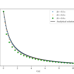
Numerical solutions of initial value problems aim at finding the solutions $\boldsymbol{x}(t)$ of the differential equations over a given interval $t \in\left[t_{0}, t_{\mathrm{n}}\right]$ in a numerical format. The quantity $t_{\mathrm{n}}$ is referred to as the terminal time. The numerical solution reliably finds how the state vector evolves from the given initial state vector $\boldsymbol{x}{0}$ in the predefined interval $t \in\left[t{0}, t_{\mathrm{n}}\right]$.
It can be seen from the initial value problem model that if the differential equations are provided in the first-order explicit form, numerical methods can be used to find the solutions of the equations. On the contrary to the analytical method, numerical methods do not significantly change when the format of differential equations changes. It will be shown in later chapters that even if the equations are not provided in the first-order explicit form, conversions can be made such that numerical solvers can still be used to solve the equations.
数学代写|微分方程代写differential equation代考|Existence and uniqueness of solutions
Two important theorems are presented in the differential equation theory to describe the existence and uniqueness of the solutions. The two theorems are listed below, ${ }^{[8]}$ with some necessary illustrations.
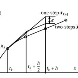
Theorem 3.1 (Existence theorem). Assuming that $f(t, x(t))$ is continuous in the rectangular region $a0$, such that in the interval $t_{0}-\epsilon<t<t_{0}+\epsilon$, the function $x(t)$ satisfies (3.1.1).
In simple terms, if $f(t, x(t))$ is a continuous function, there exists solutions to the initial value problems. However, this does not imply that if the function is not continuous, there is no solutions.
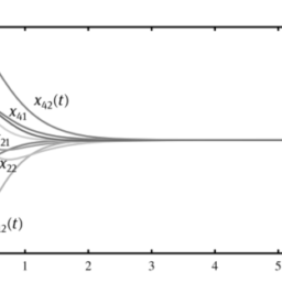
Theorem $3.2$ (Uniqueness theorem). Assume that $f(t, x(t))$ is continuous over the rectangular region $a0$, such that in the time interval $t_{0}-\epsilon<t<t_{0}+\epsilon$, if the equation has two solutions $x_{1}(t)$ and $x_{2}(t)$, one has $x_{1}(t)=x_{2}(t)$. In other words, the solution is unique.

微分方程代写
数学代写|微分方程代写DIFFERENTIAL EQUATION代考|MATHEMATICAL FORMS OF INITIAL VALUE PROBLEMS
本节介绍一阶显式微分方程格式,可以作为后面介绍的数值算法的基础。
定义 3.1。一阶显式微分方程的数学模型由下式给出
$$
\boldsymbol{x}^{\prime}(t)=\boldsymbol{f}(t, \boldsymbol{x}(t))
$$
where the vector $\boldsymbol{x}(t)=\left[x_{1}(t), x_{2}(t), \ldots, x_{n}(t)\right]^{\mathrm{T}}$ is known as the state vector, and the function vector $\boldsymbol{f}(\cdot)=\left[f_{1}(\cdot), f_{2}(\cdot), \ldots, f_{n}(\cdot)\right]^{\mathrm{T}}$ i要解决,这个问题被认为是一个初值问题。
初值问题的数值解旨在找到解X(吨)给定区间内的微分方程吨∈[吨0,吨n]以数字格式。数量吨n称为终端时间。数值解可靠地找到状态向量如何从给定的初始状态向量 $\boldsymbol{x} {0}一世n吨H和pr和d和F一世n和d一世n吨和rv一种一世t \in\left[t {0}, t_{\mathrm{n}}\right]$。
从初值问题模型可以看出,如果微分方程以一阶显式形式提供,则可以使用数值方法求解方程组。与解析方法相反,数值方法在微分方程的格式发生变化时不会发生显着变化。在后面的章节中将显示,即使方程没有以一阶显式形式提供,也可以进行转换,以便仍然可以使用数值求解器来求解方程。
数学代写|微分方程代写DIFFERENTIAL EQUATION代考|EXISTENCE AND UNIQUENESS OF SOLUTIONS
微分方程理论中提出了两个重要的定理来描述解的存在性和唯一性。下面列出了这两个定理,[8]附上一些必要的插图。
定理 3.1和X一世s吨和nC和吨H和这r和米. 假如说F(吨,X(吨))在矩形区域内是连续的一种0,使得在区间吨0−ε<吨<吨0+ε, 功能X(吨)满足3.1.1.
简单来说,如果F(吨,X(吨))是一个连续函数,存在初值问题的解。但是,这并不意味着如果函数不连续,就没有解。
定理3.2 ün一世q你和n和ss吨H和这r和米. 假使,假设F(吨,X(吨))在矩形区域上是连续的一种0,使得在时间间隔内吨0−ε<吨<吨0+ε, 如果方程有两个解X1(吨)和X2(吨), 一个有X1(吨)=X2(吨). 换句话说,解决方案是独一无二的。

数学代写|微分方程代写differential equation代考 请认准UprivateTA™. UprivateTA™为您的留学生涯保驾护航。