如果你也在 怎样代写电动力学electrodynamics这个学科遇到相关的难题,请随时右上角联系我们的24/7代写客服。电动力学electrodynamics是物理学的一个分支,涉及到对电磁力的研究,这是一种发生在带电粒子之间的物理作用。电磁力是由电场和磁场组成的电磁场所承载的,它是诸如光这样的电磁辐射的原因。它与强相互作用、弱相互作用和引力一起,是自然界的四种基本相互作用(通常称为力)之一。
电动力学electrodynamics电磁现象是以电磁力来定义的,有时也称为洛伦兹力,它包括电和磁,是同一现象的不同表现形式。电磁力在决定日常生活中遇到的大多数物体的内部属性方面起着重要作用。原子核和其轨道电子之间的电磁吸引力将原子固定在一起。电磁力负责原子之间形成分子的化学键,以及分子间的力量。电磁力支配着所有的化学过程,这些过程是由相邻原子的电子之间的相互作用产生的。电磁学在现代技术中应用非常广泛,电磁理论是电力工程和电子学包括数字技术的基础。
my-assignmentexpert™ 电动力学electrodynamics作业代写,免费提交作业要求, 满意后付款,成绩80\%以下全额退款,安全省心无顾虑。专业硕 博写手团队,所有订单可靠准时,保证 100% 原创。my-assignmentexpert™, 最高质量的电动力学electrodynamics作业代写,服务覆盖北美、欧洲、澳洲等 国家。 在代写价格方面,考虑到同学们的经济条件,在保障代写质量的前提下,我们为客户提供最合理的价格。 由于统计Statistics作业种类很多,同时其中的大部分作业在字数上都没有具体要求,因此电动力学electrodynamics作业代写的价格不固定。通常在经济学专家查看完作业要求之后会给出报价。作业难度和截止日期对价格也有很大的影响。
想知道您作业确定的价格吗? 免费下单以相关学科的专家能了解具体的要求之后在1-3个小时就提出价格。专家的 报价比上列的价格能便宜好几倍。
my-assignmentexpert™ 为您的留学生涯保驾护航 在物理physics作业代写方面已经树立了自己的口碑, 保证靠谱, 高质且原创的电动力学electrodynamics代写服务。我们的专家在物理physics代写方面经验极为丰富,各种电动力学electrodynamics相关的作业也就用不着 说。
我们提供的电动力学electrodynamics及其相关学科的代写,服务范围广, 其中包括但不限于:
物理代写|电动力学作业代electrodynamics代考|Linear and Circular Polarization of Plane Electromagnetic Waves
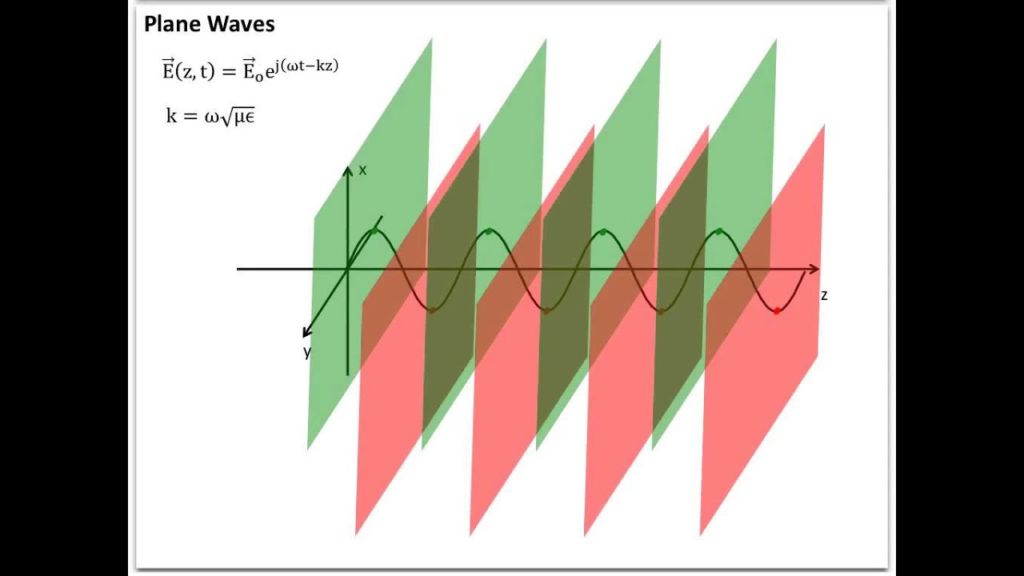
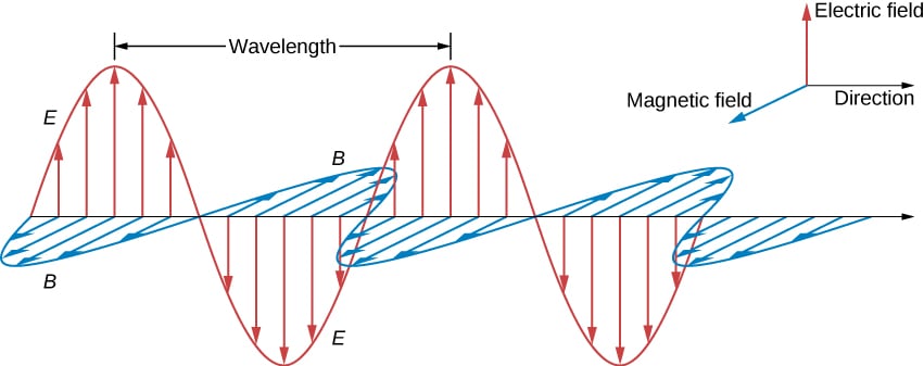
The vector nature of plane electromagnetic waves brings in new features to the wave propagation mode. These new features are related to the polarization degree of freedom of the plane electromagnetic waves. Polarization of the plane electromagnetic wave is related to the direction of oscillation of the electric field in the electromagnetic wave. Once we know the direction of wave propagation and the polarization of the wave, we practically know everything about the electromagnetic wave as the magnetic field oscillates in a direction that is mutually perpendicular to both the propagation direction and the electric field. Previously we noted two possibilities of the electric and magnetic field directions in the plane wave as
$$
\mathcal{E}=\epsilon_{1} E_{0}, \quad \mathcal{B}=\epsilon_{2} \sqrt{\mu \epsilon} E_{0}
$$
or
$$
\mathcal{E}=\epsilon_{2} E_{0}^{\prime}, \quad \mathcal{B}=-\epsilon_{1} \sqrt{\mu \epsilon} E_{0}^{\prime}
$$
Plane waves where the electric field oscillation directions are given in such a fashion, where the direction of oscillation of the electric field is fixed in time, are called linearly polarized electromagnetic waves. In the first case, the wave is linearly polarized in the direction of $\epsilon_{1}$, whereas in the second case, the wave is linearly polarized in the direction of $\epsilon_{2}$. The linearly polarized waves discussed before can be specified by the fields
$$
\mathbf{E}{1}=\epsilon{1} E_{1} e^{i(\mathbf{k} \cdot \mathbf{x}-\omega t)}, \quad \mathbf{B}{1}=\sqrt{\mu \epsilon} \frac{\mathbf{k} \times \mathbf{E}{1}}{k}
$$
or
$$
\mathbf{E}{2}=\epsilon{2} E_{2} e^{i(\mathbf{k} \cdot \mathbf{x}-\omega t)}, \quad \mathbf{B}{2}=\sqrt{\mu \epsilon} \frac{\mathbf{k} \times \mathbf{E}{2}}{k}
$$
物理代写|电动力学作业代electrodynamics代考|General Polarization Basis
The two vectors, representing two different circular polarizations, can be used to describe the most general polarization state of the plane electromagnetic wave. To verify this statement, we first introduce the two complex orthogonal unit vectors:
$$
\epsilon_{\pm}=\frac{1}{\sqrt{2}}\left(\epsilon_{1} \pm i \epsilon_{2}\right)
$$
We can find out the properties of these polarization basis. First, we see that
$$
\epsilon_{++}^{} \cdot \epsilon_{+}=\frac{1}{2}\left(\epsilon_{1}-i \epsilon_{2}\right) \cdot\left(\epsilon_{1}+i \epsilon_{2}\right)=\frac{1}{2}\left(\epsilon_{1} \cdot \epsilon_{1}+\epsilon_{2} \cdot \epsilon_{2}+i \epsilon_{1} \cdot \epsilon_{2}-i \epsilon_{2} \cdot \epsilon_{1}\right) . $$ As we know that $\boldsymbol{\epsilon}{i} \cdot \boldsymbol{\epsilon}{j}=\delta_{i j}$ where $i, j$ runs over values 1,2 , one can easily show
$$
\boldsymbol{\epsilon}{+}^{} \cdot \boldsymbol{\epsilon}{+}=1 .
$$
We can also see that
$$
\boldsymbol{\epsilon}{+}^{} \cdot \epsilon{-}=\frac{1}{2}\left(\epsilon_{1}-i \epsilon_{2}\right) \cdot\left(\epsilon_{1}-i \epsilon_{2}\right)=\frac{1}{2}\left(\epsilon_{1} \cdot \epsilon_{1}-\epsilon_{2} \cdot \epsilon_{2}-i \epsilon_{1} \cdot \epsilon_{2}-i \epsilon_{2} \cdot \epsilon_{1}\right)=0
$$
In general, we can write
$$
\boldsymbol{\epsilon}{+}^{} \cdot \boldsymbol{\epsilon}{+}=\boldsymbol{\epsilon}{-}^{} \cdot \boldsymbol{\epsilon}{-}=1, \quad \text { and } \quad \boldsymbol{\epsilon}{+}^{} \cdot \boldsymbol{\epsilon}{-}=\boldsymbol{\epsilon}{-}^{*} \cdot \boldsymbol{\epsilon}{+}=0
$$
showing that these vectors form an orthonormal set of basis vectors. Of course, we have another condition which define these basis vectors
$$
\boldsymbol{\epsilon}_{\pm} \cdot \hat{\mathbf{n}}=0
$$
物理代写|电动力学作业代ELECTRODYNAMICS代考|Stokes Parameters
The polarization content of the plane electromagnetic wave can be known if we can write it down in the form
$$
\mathbf{E}(\mathbf{x}, t)=\left(\boldsymbol{\epsilon}{1} E{1}+\boldsymbol{\epsilon}{2} E{2}\right) e^{i(\mathbf{k} \cdot \mathbf{x}-\omega t)},
$$
showing that the wave is plane polarized, or in the form
$$
\mathbf{E}(\mathbf{x}, t)=\left(E_{+} \boldsymbol{\epsilon}{+}+E{-} \boldsymbol{\epsilon}{-}\right) e^{i(\mathbf{k} \cdot \mathbf{x}-\omega t)} $$ showing that it is elliptically polarized. If we know the pairs $\left(E{1}, E_{2}\right)$ or $\left(E_{+}, E_{-}\right)$, then we know fully the polarization state of the electromagnetic wave. In reality, the converse problem arises. From astrophysical sources or some other sources, we only know that the electric field is of the form
$$
\mathbf{E}(\mathbf{x}, t)=\mathcal{E} e^{i(\mathbf{k} \cdot \mathbf{x}-\omega t)}, \quad \mathbf{B}(\mathbf{x}, t)=\mathcal{B} e^{i(\mathbf{k} \cdot \mathbf{x}-\omega t)},
$$
which are not written in the polarization basis. The problem now is how do we know about the polarization state of light from this information. We require to measure some quantities related to the incoming light beam to understand the proper polarization basis of the incoming plane waves. We know that light can be linearly polarized or elliptically polarized, but we do not know exactly in which state of polarization the light beam is.
To tackle this problem, the Stokes parameters become useful. These parameters are quadratic in the field strength and can be determined through the intensity measurements and polarizers. Stokes parameters are important as they help us to opine about the vectorial nature of light from intensity measurements. Suppose we are looking at light traveling along $z$ direction, then the Stokes parameters are related to the basic quantities
$$
\epsilon_{1} \cdot \mathbf{E}, \quad \boldsymbol{\epsilon}{2} \cdot \mathbf{E}, \quad \epsilon{+}^{} \cdot \mathbf{E}, \quad \epsilon_{-}^{} \cdot \mathbf{E}
$$
电动力学代写
物理代写|电动力学作业代ELECTRODYNAMICS代考|LINEAR AND CIRCULAR POLARIZATION OF PLANE ELECTROMAGNETIC WAVES
平面电磁波的矢量性质为波传播模式带来了新的特征。这些新特征与平面电磁波的极化自由度有关。平面电磁波的极化与电磁波中电场的振荡方向有关。一旦我们知道了波的传播方向和波的极化,我们实际上就知道了关于电磁波的一切,因为磁场在一个与传播方向和电场相互垂直的方向上振荡。之前我们注意到平面波中电场和磁场方向的两种可能性:
$$
\mathcal{E}=\epsilon_{1} E_{0}, \quad \mathcal{B}=\epsilon_{2} \sqrt{\mu \epsilon} E_{0}
$$
or
$$
\mathcal{E}=\epsilon_{2} E_{0}^{\prime}, \quad \mathcal{B}=-\epsilon_{1} \sqrt{\mu \epsilon} E_{0}^{\prime}
$$
Plane waves where the electric field oscillation directions are given in such a fashion, where the direction of oscillation of the electric field is fixed in time, are called linearly polarized electromagnetic waves. In the first case, the wave is linearly polarized in the direction of $\epsilon_{1}$, whereas in the second case, the wave is linearly polarized in the direction of $\epsilon_{2}$. The linearly polarized waves discussed before can be specified by the fields
$$
\mathbf{E}{1}=\epsilon{1} E_{1} e^{i(\mathbf{k} \cdot \mathbf{x}-\omega t)}, \quad \mathbf{B}{1}=\sqrt{\mu \epsilon} \frac{\mathbf{k} \times \mathbf{E}{1}}{k}
$$
or
$$
\mathbf{E}{2}=\epsilon{2} E_{2} e^{i(\mathbf{k} \cdot \mathbf{x}-\omega t)}, \quad \mathbf{B}{2}=\sqrt{\mu \epsilon} \frac{\mathbf{k} \times \mathbf{E}{2}}{k}
$$
物理代写|电动力学作业代ELECTRODYNAMICS代考|GENERAL POLARIZATION BASIS
这两个向量,代表两种不同的圆极化,可以用来描述平面电磁波最一般的极化状态。为了验证这个说法,我们首先引入两个复正交单位向量:
ε±=12(ε1±一世ε2)
我们可以找出这些极化基的性质。首先,我们看到
$$
\epsilon_{\pm}=\frac{1}{\sqrt{2}}\left(\epsilon_{1} \pm i \epsilon_{2}\right)
$$
We can find out the properties of these polarization basis. First, we see that
$$
\epsilon_{++}^{} \cdot \epsilon_{+}=\frac{1}{2}\left(\epsilon_{1}-i \epsilon_{2}\right) \cdot\left(\epsilon_{1}+i \epsilon_{2}\right)=\frac{1}{2}\left(\epsilon_{1} \cdot \epsilon_{1}+\epsilon_{2} \cdot \epsilon_{2}+i \epsilon_{1} \cdot \epsilon_{2}-i \epsilon_{2} \cdot \epsilon_{1}\right) . $$ As we know that $\boldsymbol{\epsilon}{i} \cdot \boldsymbol{\epsilon}{j}=\delta_{i j}$ where $i, j$ runs over values 1,2 , one can easily show
$$
\boldsymbol{\epsilon}{+}^{} \cdot \boldsymbol{\epsilon}{+}=1 .
$$
We can also see that
$$
\boldsymbol{\epsilon}{+}^{} \cdot \epsilon{-}=\frac{1}{2}\left(\epsilon_{1}-i \epsilon_{2}\right) \cdot\left(\epsilon_{1}-i \epsilon_{2}\right)=\frac{1}{2}\left(\epsilon_{1} \cdot \epsilon_{1}-\epsilon_{2} \cdot \epsilon_{2}-i \epsilon_{1} \cdot \epsilon_{2}-i \epsilon_{2} \cdot \epsilon_{1}\right)=0
$$
In general, we can write
$$
\boldsymbol{\epsilon}{+}^{} \cdot \boldsymbol{\epsilon}{+}=\boldsymbol{\epsilon}{-}^{} \cdot \boldsymbol{\epsilon}{-}=1, \quad \text { and } \quad \boldsymbol{\epsilon}{+}^{} \cdot \boldsymbol{\epsilon}{-}=\boldsymbol{\epsilon}{-}^{*} \cdot \boldsymbol{\epsilon}{+}=0
$$
showing that these vectors form an orthonormal set of basis vectors. Of course, we have another condition which define these basis vectors
$$
\boldsymbol{\epsilon}_{\pm} \cdot \hat{\mathbf{n}}=0
$$
物理代写|电动力学作业代ELECTRODYNAMICS代考|STOKES PARAMETERS
平面电磁波的极化内容可以写成
$$
\mathbf{E}(\mathbf{x}, t)=\left(\boldsymbol{\epsilon}{1} E{1}+\boldsymbol{\epsilon}{2} E{2}\right) e^{i(\mathbf{k} \cdot \mathbf{x}-\omega t)},
$$
showing that the wave is plane polarized, or in the form
$$
\mathbf{E}(\mathbf{x}, t)=\left(E_{+} \boldsymbol{\epsilon}{+}+E{-} \boldsymbol{\epsilon}{-}\right) e^{i(\mathbf{k} \cdot \mathbf{x}-\omega t)} $$ showing that it is elliptically polarized. If we know the pairs $\left(E{1}, E_{2}\right)$ or $\left(E_{+}, E_{-}\right)$, then we know fully the polarization state of the electromagnetic wave. In reality, the converse problem arises. From astrophysical sources or some other sources, we only know that the electric field is of the form
$$
\mathbf{E}(\mathbf{x}, t)=\mathcal{E} e^{i(\mathbf{k} \cdot \mathbf{x}-\omega t)}, \quad \mathbf{B}(\mathbf{x}, t)=\mathcal{B} e^{i(\mathbf{k} \cdot \mathbf{x}-\omega t)},
$$
其中没有写在极化基础上。现在的问题是我们如何从这些信息中了解光的偏振状态。我们需要测量与入射光束相关的一些量,以了解入射平面波的正确偏振基础。我们知道光可以是线性偏振或椭圆偏振,但我们并不确切知道光束处于哪种偏振状态。
为了解决这个问题,斯托克斯参数变得有用。这些参数在场强中是二次的,可以通过强度测量和偏振器来确定。斯托克斯参数很重要,因为它们帮助我们从强度测量中判断光的矢量性质。假设我们正在观察沿行传播的光和方向,则斯托克斯参数与基本量有关
$$
\mathbf{E}{2}=\epsilon{2} E_{2} e^{i(\mathbf{k} \cdot \mathbf{x}-\omega t)}, \quad \mathbf{B}{2}=\sqrt{\mu \epsilon} \frac{\mathbf{k} \times \mathbf{E}{2}}{k}
$$

物理代写|电动力学作业代写electrodynamics代考 请认准UprivateTA™. UprivateTA™为您的留学生涯保驾护航。