如果你也在 怎样代写电动力学electrodynamics这个学科遇到相关的难题,请随时右上角联系我们的24/7代写客服。电动力学electrodynamics是物理学的一个分支,涉及到对电磁力的研究,这是一种发生在带电粒子之间的物理作用。电磁力是由电场和磁场组成的电磁场所承载的,它是诸如光这样的电磁辐射的原因。它与强相互作用、弱相互作用和引力一起,是自然界的四种基本相互作用(通常称为力)之一。
电动力学electrodynamics电磁现象是以电磁力来定义的,有时也称为洛伦兹力,它包括电和磁,是同一现象的不同表现形式。电磁力在决定日常生活中遇到的大多数物体的内部属性方面起着重要作用。原子核和其轨道电子之间的电磁吸引力将原子固定在一起。电磁力负责原子之间形成分子的化学键,以及分子间的力量。电磁力支配着所有的化学过程,这些过程是由相邻原子的电子之间的相互作用产生的。电磁学在现代技术中应用非常广泛,电磁理论是电力工程和电子学包括数字技术的基础。
my-assignmentexpert™ 电动力学electrodynamics作业代写,免费提交作业要求, 满意后付款,成绩80\%以下全额退款,安全省心无顾虑。专业硕 博写手团队,所有订单可靠准时,保证 100% 原创。my-assignmentexpert™, 最高质量的电动力学electrodynamics作业代写,服务覆盖北美、欧洲、澳洲等 国家。 在代写价格方面,考虑到同学们的经济条件,在保障代写质量的前提下,我们为客户提供最合理的价格。 由于统计Statistics作业种类很多,同时其中的大部分作业在字数上都没有具体要求,因此电动力学electrodynamics作业代写的价格不固定。通常在经济学专家查看完作业要求之后会给出报价。作业难度和截止日期对价格也有很大的影响。
想知道您作业确定的价格吗? 免费下单以相关学科的专家能了解具体的要求之后在1-3个小时就提出价格。专家的 报价比上列的价格能便宜好几倍。
my-assignmentexpert™ 为您的留学生涯保驾护航 在物理physics作业代写方面已经树立了自己的口碑, 保证靠谱, 高质且原创的电动力学electrodynamics代写服务。我们的专家在物理physics代写方面经验极为丰富,各种电动力学electrodynamics相关的作业也就用不着 说。
我们提供的电动力学electrodynamics及其相关学科的代写,服务范围广, 其中包括但不限于:
物理代写|电动力学作业代electrodynamics代考|Magnetostatics
The equations that govern the boundary value problems in presence of magnetized macroscopic linear media are as follows:
$$
\begin{aligned}
\nabla \cdot \mathbf{B} &=0 \
\nabla \times \mathbf{H} &=\frac{4 \pi}{c} \mathbf{J}
\end{aligned}
$$
The vector fields $\mathbf{B}, \mathbf{H}$ and $\mathbf{M}$ are related to each other by the following set of equations:
$$
\begin{aligned}
\mathbf{B} &=\mathbf{H}+4 \pi \mathbf{M} \
\mathbf{M} &=\chi_{m} \mathbf{H} \
\mathbf{B} &=\mu \mathbf{H}
\end{aligned}
$$
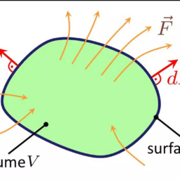
Typically, the spatial distribution of $\mathbf{M}$ inside the macroscopic object of volume $V$ bounded by surface $\partial V$ is given, which is ‘frozen’ in time. We are particularly interested in situations where the free current $\mathbf{J}{f}=0$, which means $\nabla \times \mathbf{H}=0$ everywhere. In such cases, H can be expressed as a gradient of ‘magnetic’ scalar potential $\Phi{M}$ defined as
$$
\mathbf{H}=-\nabla \Phi_{M} .
$$
It then follows from Eqs. (3.127) and (3.129)
$$
\nabla \cdot \mathbf{H}=-4 \pi \nabla \cdot \mathbf{M}
$$
Combining Eqs. (3.132) and (3.133), we finally arrive at the following equation:
$$
\nabla^{2} \Phi_{M}=4 \pi \nabla \cdot \mathbf{M}=-4 \pi \rho_{M} .
$$
This is strikingly similar to the Poisson equation we encountered in electrostatics, albeit with an effective or fictitious ‘magnetic charge’ $\rho_{M}=-\nabla \cdot \mathbf{M}$. Since we are already familiar with the formal solution of the Poisson equation for electrostatics, ${ }^{10}$ we can readily write down the solution in absence of boundaries as
$$
\Phi_{M}(\mathbf{x})=\int \frac{-\nabla^{\prime} \cdot \mathbf{M}\left(\mathbf{x}^{\prime}\right)}{\left|\mathbf{x}-\mathbf{x}^{\prime}\right|} d^{3} x^{\prime}
$$
Further, if $\mathbf{M}$ is well behaved and localized,
$$
\Phi_{M}(\mathbf{x})=-\int \nabla^{\prime} \cdot \frac{\mathbf{M}\left(\mathbf{x}^{\prime}\right)}{\left|\mathbf{x}-\mathbf{x}^{\prime}\right|} d^{3} x^{\prime}+\int \nabla^{\prime} \frac{1}{\left|\mathbf{x}-\mathbf{x}^{\prime}\right|} \cdot \mathbf{M}\left(\mathbf{x}^{\prime}\right) d^{3} x^{\prime} .
$$
Interchanging primed and unprimed variables in the gradient term, we can write
$$
\nabla^{\prime} \frac{1}{\left|\mathbf{x}-\mathbf{x}^{\prime}\right|}=-\nabla \frac{1}{\left|\mathbf{x}-\mathbf{x}^{\prime}\right|}
$$
Since in the second term, the differentiation is with respect to unprimed variable, we can take it outside the integral which is over primed variables and write
$$
\Phi_{M}(\mathbf{x})=-\int \nabla^{\prime} \cdot \frac{\mathbf{M}\left(\mathbf{x}^{\prime}\right)}{\left|\mathbf{x}-\mathbf{x}^{\prime}\right|} d^{3} x^{\prime}-\nabla \cdot \int \frac{\mathbf{M}\left(\mathbf{x}^{\prime}\right)}{\left|\mathbf{x}-\mathbf{x}^{\prime}\right|} d^{3} x^{\prime}
$$
物理代写|电动力学作业代electrodynamics代考|A Uniformly Magnetized Sphere
We consider a uniformly magnetized sphere of radius $R$ (Fig. 3.8) without any free current. Outside the sphere, the magnetization vanishes abruptly. Inside the sphere,
$$
\mathbf{M}=M \hat{\mathbf{z}} .
$$
In this case, the volume magnetic charge density $\rho_{M}=-\nabla \cdot \mathbf{M}=0$ and the surface magnetic charge density $\sigma_{M}=\mathbf{M} \cdot \hat{\mathbf{n}}=M \cos \theta$.
Since $\rho_{M}=0$, the magnetic scalar potential $\Phi_{M}$ satisfies the Laplace equation not just outside but inside the sphere as well. We want to find out the potential in these two regions (as we have already done in electrostatics), albeit using the boundary conditions of magnetostatics. Again, the azimuthal symmetry in the problem suggests that the solution must be an expansion in terms of the Legendre polynomials. Inside the sphere, for $rR$,
$$
\Phi_{M}^{\text {out }}(r, \theta)=\sum_{l=0}^{\infty} B_{l} r^{-(l+1)} P_{l}(\cos \theta)
$$
Again, inside the sphere,
$$
\begin{aligned}
&\mathbf{H}{\text {in }}=-\nabla \Phi{M}^{\text {in }}, \
&\mathbf{B}{\text {in }}=\mathbf{H}{\text {in }}+4 \pi M \hat{\mathbf{z}} .
\end{aligned}
$$
Outside the sphere,
$$
\begin{aligned}
\mathbf{H}{\text {out }} &=-\nabla \Phi{M}^{\text {out }} \
\mathbf{B}{\text {out }} &=\mathbf{H}{\text {out }}
\end{aligned}
$$
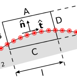
We now write down the boundary conditions. From Eq. (3.123), we have
$$
\left.\frac{\partial \Phi_{M}^{\mathrm{in}}}{\partial r}\right|{r=R}-\left.\frac{\partial \Phi{M}^{\text {out }}}{\partial r}\right|{r=R}=4 \pi M \cos \theta . $$ Moreover, since there is no free charge current, Eq. (3.125) implies that the tangential component of $\mathbf{H}$ is continuous at the surface of the sphere $$ \left.\frac{\partial \Phi{M}^{\text {in }}}{\partial \theta}\right|{r=R}=\left.\frac{\partial \Phi{M}^{\text {out }}}{\partial \theta}\right|_{r=R} .
$$
电动力学代写
物理代写|电动力学作业代ELECTRODYNAMICS代考|MAGNETOSTATICS
控制存在磁化宏观线性介质的边值问题的方程如下:
∇⋅乙=0 ∇×H=4圆周率CĴ
向量场乙,H和米通过以下一组方程相互关联:乙=H+4圆周率米 米=χ米H 乙=μH
通常,空间分布米在体积的宏观对象内部五以曲面为界∂五被给定,它被及时“冻结”。我们对自由电流 $\mathbf{J} {f}=0的情况特别感兴趣, $\mathbf{J}{f}=0$, which means $\nabla \times \mathbf{H}=0$ everywhere. In such cases, H can be expressed as a gradient of ‘magnetic’ scalar potential $\Phi{M}$ defined as
$$
\mathbf{H}=-\nabla \Phi_{M} .
$$
It then follows from Eqs. (3.127) and (3.129)
$$
\nabla \cdot \mathbf{H}=-4 \pi \nabla \cdot \mathbf{M}
$$
Combining Eqs. (3.132) and (3.133), we finally arrive at the following equation:
$$
\nabla^{2} \Phi_{M}=4 \pi \nabla \cdot \mathbf{M}=-4 \pi \rho_{M} .
$$
This is strikingly similar to the Poisson equation we encountered in electrostatics, albeit with an effective or fictitious ‘magnetic charge’ $\rho_{M}=-\nabla \cdot \mathbf{M}$. Since we are already familiar with the formal solution of the Poisson equation for electrostatics, ${ }^{10}$ we can readily write down the solution in absence of boundaries as
$$
\Phi_{M}(\mathbf{x})=\int \frac{-\nabla^{\prime} \cdot \mathbf{M}\left(\mathbf{x}^{\prime}\right)}{\left|\mathbf{x}-\mathbf{x}^{\prime}\right|} d^{3} x^{\prime}
$$
Further, if $\mathbf{M}$ is well behaved and localized,
$$
\Phi_{M}(\mathbf{x})=-\int \nabla^{\prime} \cdot \frac{\mathbf{M}\left(\mathbf{x}^{\prime}\right)}{\left|\mathbf{x}-\mathbf{x}^{\prime}\right|} d^{3} x^{\prime}+\int \nabla^{\prime} \frac{1}{\left|\mathbf{x}-\mathbf{x}^{\prime}\right|} \cdot \mathbf{M}\left(\mathbf{x}^{\prime}\right) d^{3} x^{\prime} .
$$
Interchanging primed and unprimed variables in the gradient term, we can write
$$
\nabla^{\prime} \frac{1}{\left|\mathbf{x}-\mathbf{x}^{\prime}\right|}=-\nabla \frac{1}{\left|\mathbf{x}-\mathbf{x}^{\prime}\right|}
$$
Since in the second term, the differentiation is with respect to unprimed variable, we can take it outside the integral which is over primed variables and write
$$
\Phi_{M}(\mathbf{x})=-\int \nabla^{\prime} \cdot \frac{\mathbf{M}\left(\mathbf{x}^{\prime}\right)}{\left|\mathbf{x}-\mathbf{x}^{\prime}\right|} d^{3} x^{\prime}-\nabla \cdot \int \frac{\mathbf{M}\left(\mathbf{x}^{\prime}\right)}{\left|\mathbf{x}-\mathbf{x}^{\prime}\right|} d^{3} x^{\prime}
$$
物理代写|电动力学作业代ELECTRODYNAMICS代考|A UNIFORMLY MAGNETIZED SPHERE
我们考虑一个半径为均匀磁化的球体R F一世G.3.8没有任何自由电流。在球体之外,磁化强度突然消失。球体内,
米=米和^.
在这种情况下,体积磁荷密度ρ米=−∇⋅米=0和表面磁荷密度σ米=米⋅n^=米某物θ.
自从ρ米=0, 磁标量势披米不仅在球体外而且在球体内也满足拉普拉斯方程。我们想找出这两个地区的潜力一种s在和H一种v和一种一世r和一种d是d这n和一世n和一世和C吨r这s吨一种吨一世Cs,尽管使用了静磁学的边界条件。再一次,问题中的方位角对称性表明解决方案必须是勒让德多项式的展开。在球体内,对于rR,披米出去 (r,θ)=∑一世=0∞乙一世r−(一世+1)磷一世(某物θ)
同样,在球体内,
$$
\begin{aligned}
&\mathbf{H}{\text {in }}=-\nabla \Phi{M}^{\text {in }}, \
&\mathbf{B}{\text {in }}=\mathbf{H}{\text {in }}+4 \pi M \hat{\mathbf{z}} .
\end{aligned}
$$
Outside the sphere,
$$
\begin{aligned}
\mathbf{H}{\text {out }} &=-\nabla \Phi{M}^{\text {out }} \
\mathbf{B}{\text {out }} &=\mathbf{H}{\text {out }}
\end{aligned}
$$
We now write down the boundary conditions. From Eq. (3.123), we have
$$
\left.\frac{\partial \Phi_{M}^{\mathrm{in}}}{\partial r}\right|{r=R}-\left.\frac{\partial \Phi{M}^{\text {out }}}{\partial r}\right|{r=R}=4 \pi M \cos \theta . $$ Moreover, since there is no free charge current, Eq. (3.125) implies that the tangential component of $\mathbf{H}$ is continuous at the surface of the sphere $$ \left.\frac{\partial \Phi{M}^{\text {in }}}{\partial \theta}\right|{r=R}=\left.\frac{\partial \Phi{M}^{\text {out }}}{\partial \theta}\right|_{r=R} .
$$tial \theta}\right|_{r=R} 。
$$

物理代写|电动力学作业代写electrodynamics代考 请认准UprivateTA™. UprivateTA™为您的留学生涯保驾护航。