如果你也在 怎样代写电动力学electrodynamics这个学科遇到相关的难题,请随时右上角联系我们的24/7代写客服。电动力学electrodynamics是物理学的一个分支,涉及到对电磁力的研究,这是一种发生在带电粒子之间的物理作用。电磁力是由电场和磁场组成的电磁场所承载的,它是诸如光这样的电磁辐射的原因。它与强相互作用、弱相互作用和引力一起,是自然界的四种基本相互作用(通常称为力)之一。
电动力学electrodynamics电磁现象是以电磁力来定义的,有时也称为洛伦兹力,它包括电和磁,是同一现象的不同表现形式。电磁力在决定日常生活中遇到的大多数物体的内部属性方面起着重要作用。原子核和其轨道电子之间的电磁吸引力将原子固定在一起。电磁力负责原子之间形成分子的化学键,以及分子间的力量。电磁力支配着所有的化学过程,这些过程是由相邻原子的电子之间的相互作用产生的。电磁学在现代技术中应用非常广泛,电磁理论是电力工程和电子学包括数字技术的基础。
my-assignmentexpert™ 电动力学electrodynamics作业代写,免费提交作业要求, 满意后付款,成绩80\%以下全额退款,安全省心无顾虑。专业硕 博写手团队,所有订单可靠准时,保证 100% 原创。my-assignmentexpert™, 最高质量的电动力学electrodynamics作业代写,服务覆盖北美、欧洲、澳洲等 国家。 在代写价格方面,考虑到同学们的经济条件,在保障代写质量的前提下,我们为客户提供最合理的价格。 由于统计Statistics作业种类很多,同时其中的大部分作业在字数上都没有具体要求,因此电动力学electrodynamics作业代写的价格不固定。通常在经济学专家查看完作业要求之后会给出报价。作业难度和截止日期对价格也有很大的影响。
想知道您作业确定的价格吗? 免费下单以相关学科的专家能了解具体的要求之后在1-3个小时就提出价格。专家的 报价比上列的价格能便宜好几倍。
my-assignmentexpert™ 为您的留学生涯保驾护航 在物理physics作业代写方面已经树立了自己的口碑, 保证靠谱, 高质且原创的电动力学electrodynamics代写服务。我们的专家在物理physics代写方面经验极为丰富,各种电动力学electrodynamics相关的作业也就用不着 说。
我们提供的电动力学electrodynamics及其相关学科的代写,服务范围广, 其中包括但不限于:
物理代写|电动力学作业代electrodynamics代考|Biot-Savart Law of Magnetostatics
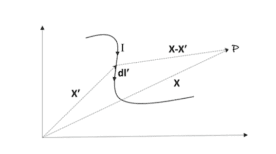
Equivalent to Coulomb’s law in electrostatics is the Biot-Savart law of magnetostatics which is applicable not just for steady current but also for quasi stationary current. According to the Biot-Savart law, the magnetic field due to a current carrying wire is given by
$$
\mathbf{B}(\mathbf{x})=\frac{1}{c} \int I \mathbf{d l}^{\prime} \times \frac{\mathbf{x}-\mathbf{x}^{\prime}}{\left|\mathbf{x}-\mathbf{x}^{\prime}\right|^{3}}
$$
Here, the integration is along the current path (Fig. 1.4).
The expression can be extended to surface current $\mathbf{K}\left(\mathbf{x}^{\prime}\right)$ and volume current $\mathbf{J}\left(\mathbf{x}^{\prime}\right)$ by replacing $I \mathbf{d l}$ with $\mathbf{K}\left(\mathbf{x}^{\prime}\right) d a^{\prime}$ and $\mathbf{J}\left(\mathbf{x}^{\prime}\right) d^{3} x^{\prime}$, respectively, in Eq. (1.49).
What will be the magnetic field due to a point charge $q$ moving with uniform velocity $\mathbf{v}$ ? A naive expectation, using the Biot-Savart law by pretending that a point charge in uniform motion does constitute a steady current (as pointed out earlier, this is not true), gives
$$
\mathbf{B}(\mathbf{x})=\frac{1}{c} q \mathbf{v} \times \frac{\mathbf{x}-\mathbf{x}^{\prime}}{\left|\mathbf{x}-\mathbf{x}^{\prime}\right|^{3}}
$$
It turns out that the expression is correct for charges with velocities that are small compared to the speed of light. However, a proper derivation of the expression involves using relativistic transformation of fields and then taking the non-relativistic limit. This will be discussed later in the book.
Similar to the electric field, the superposition principle applies to the magnetic field as well. It states that for a collection of source currents, the net magnetic field is the vector sum of fields due to each of the source currents measured separately.
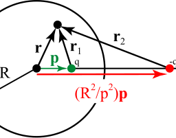
As an illustration, let us calculate the force between two current loops (Fig. 1.5). This is instructive as we will have to use the Biot-Savart law to calculate the magnetic field at one current loop due to the other and additionally the force law of Eq. (1.42). We adopted the general convention that the position vectors of source elements are labeled by primed variables and the position vectors of the observation points by unprimed variables. However, in this case, we note that the position vector of the source element in the one loop is the position vector of the observation point for the other and vice versa.
物理代写|电动力学作业代electrodynamics代考|General Derivation of Ampere’s Law
We start from the Biot-Savart law for magnetic field due to a volume current distribution $\mathbf{J}\left(\mathbf{r}^{\prime}\right)$
$$
\mathbf{B}(\mathbf{x})=\frac{1}{c} \int \mathbf{J}\left(\mathbf{x}^{\prime}\right) \times \frac{\mathbf{x}-\mathbf{x}^{\prime}}{\left|\mathbf{x}-\mathbf{x}^{\prime}\right|^{3}} d^{3} x^{\prime} .
$$
At this point, we ask a legitimate question. We know that the divergence of electric field at a point in space is non-zero if the charge density is non-zero at that point. What is the divergence of a magnetic field? For this, we take the divergence on both sides of Eq. (1.56). Before explicitly performing the calculation, we keep in mind that the integration is over the primed variables representing sources, while the operation $\nabla$ is with respect to unprimed variables representing observation points and consequently
$$
\nabla \cdot \mathbf{J}\left(\mathbf{x}^{\prime}\right) \times \frac{\mathbf{x}-\mathbf{x}^{\prime}}{\left|\mathbf{x}-\mathbf{x}^{\prime}\right|^{3}}=\frac{\mathbf{x}-\mathbf{x}^{\prime}}{\left|\mathbf{x}-\mathbf{x}^{\prime}\right|^{3}} \cdot\left(\nabla \times \mathbf{J}^{\prime}\right)-\mathbf{J}^{\prime} \cdot\left(\nabla \times \frac{\mathbf{x}-\mathbf{x}^{\prime}}{\left|\mathbf{x}-\mathbf{x}^{\prime}\right|^{3}}\right)
$$
The second term on the right-hand side of the equation vanishes as this is exactly similar to the case of electrostatic field. What about the first term? Here, $\mathbf{J}^{\prime}$ is a function of the primed variable while the operation $\nabla$ is over unprimed variables. Therefore, the first term vanishes as well. We can now express the Biot-Savart law in differential form as follows:
$$
\nabla \cdot \mathbf{B}(\mathbf{x})=0
$$
Compare the equation with the corresponding one for the electric field. Unlike the electric field, the divergence of the magnetic field at each point in space vanishes. This tells us that there is no monopole term in the multipole expansion of magnetic sources or, in other words, there are no sources or sinks in the magnetic field lines.
We can also rewrite Eq. (1.56) in the following way:
$$
\begin{aligned}
\mathbf{B}(\mathbf{r}) &=-\frac{1}{c} \int \mathbf{J}\left(\mathbf{x}^{\prime}\right) \times \nabla \frac{1}{\left|\mathbf{x}-\mathbf{x}^{\prime}\right|} \
&=\frac{1}{c} \nabla \times \int \frac{\mathbf{J}\left(\mathbf{x}^{\prime}\right)}{\left|\mathbf{x}-\mathbf{x}^{\prime}\right|} d^{3} x^{\prime}
\end{aligned}
$$
Here, we have used standard vector identity $\nabla \times(\phi \mathbf{G})=\nabla \phi \times \mathbf{G}+\phi \nabla \times \mathbf{G}$. We have also used $\nabla \frac{1}{\left|\mathbf{x}-\mathbf{x}^{\prime}\right|}=-\frac{\mathbf{x}-\mathbf{x}^{\prime}}{\left|\mathbf{x}-\mathbf{x}^{\prime}\right|^{3}}$ and $\nabla \times \mathbf{J}\left(\mathbf{x}^{\prime}\right)=0$. Since $\nabla$ is over unprimed variables, $\nabla \times \mathbf{J}\left(\mathbf{x}^{\prime}\right)$ vanishes.
We now define the ‘vector potential’ A for magnetostatics as
$$
\mathbf{A}(\mathbf{x})=\frac{1}{c} \int \frac{\mathbf{J}\left(\mathbf{x}^{\prime}\right)}{\left|\mathbf{x}-\mathbf{x}^{\prime}\right|} d^{3} x^{\prime},
$$
so that the magnetic field can be expressed as $\mathbf{B}=\nabla \times \mathbf{A}$.
物理代写|电动力学作业代ELECTRODYNAMICS代考|Vector Potential
We have already defined the vector potential $\mathbf{A}(\mathbf{x})$ in Eq. (1.61). Such a definition is not completely free from arbitrariness. Since the magnetic field $\mathbf{B}$ is divergence-free everywhere, it automatically follows that $\mathbf{B}$ can be expressed as curl of some vector field $\mathbf{A}$ as
$$
\mathbf{B}=\nabla \times \mathbf{A} .
$$
The most general expression of $\mathbf{A}$, therefore, includes an added term which is a gradient of an arbitrary scalar function $\chi(\mathbf{x})$, as curl of gradient of any scalar function goes to zero:
$$
\mathbf{A}(\mathbf{x})=\frac{1}{c} \int \frac{\mathbf{J}\left(\mathbf{x}^{\prime}\right)}{\left|\mathbf{x}-\mathbf{x}^{\prime}\right|}+\nabla \chi(\mathbf{x})
$$
For a given magnetic field $\mathbf{B}$, the choice of vector potential is not unique. It can undergo the following transformation, without leading to any change in $\mathbf{B}$ :
$$
\mathbf{A}^{\prime} \longrightarrow \mathbf{A}+\nabla \chi
$$
Such a transformation is called gauge transformation. We shall discuss gauge transformation in greater detail later on. Here, we have a limited purpose: we choose a particular gauge so that each Cartesian component of the vector potential satisfies the Poisson equation, the solutions for which we are already familiar with. We use Eq. (1.66) to replace $\mathbf{B}$ in Eq. (1.64) and get
$$
\nabla \times(\nabla \times \mathbf{A})=\nabla(\nabla \cdot \mathbf{A})-\nabla^{2} \mathbf{A}=\frac{4 \pi}{c} \mathbf{J}
$$

电动力学代写
物理代写|电动力学作业代ELECTRODYNAMICS代考|BIOT-SAVART LAW OF MAGNETOSTATICS
与静电学中的库仑定律等效的是静磁学的 Biot-Savart 定律,它不仅适用于稳态电流,也适用于准稳态电流。根据 Biot-Savart 定律,载流导线产生的磁场由下式给出
乙(X)=1C∫一世d一世′×X−X′|X−X′|3
在这里,整合是沿着当前的路径F一世G.1.4.
该表达式可以扩展到表面电流到(X′)和体积电流Ĵ(X′)通过更换一世d一世和到(X′)d一种′和Ĵ(X′)d3X′,分别在方程式中。1.49.
点电荷产生的磁场是多少q匀速运动v? 一种天真的期望,使用 Biot-Savart 定律,假装匀速运动的点电荷确实构成稳定电流一种sp这一世n吨和d这你吨和一种r一世一世和r,吨H一世s一世sn这吨吨r你和, 给出
乙(X)=1Cqv×X−X′|X−X′|3
事实证明,该表达式对于速度小于光速的电荷是正确的。然而,表达式的适当推导涉及使用场的相对论变换,然后采用非相对论极限。这将在本书后面讨论。
与电场类似,叠加原理也适用于磁场。它指出,对于源电流的集合,净磁场是由单独测量的每个源电流引起的场的矢量和。
作为说明,让我们计算两个电流回路之间的力F一世G.1.5. 这是有启发性的,因为我们将不得不使用 Biot-Savart 定律来计算一个电流回路由于另一个电流回路的磁场,另外还有方程式的力定律。1.42. 我们采用了一般惯例,即源元素的位置向量由素变量标记,观察点的位置向量由无素变量标记。然而,在这种情况下,我们注意到一个循环中源元素的位置向量是另一个循环中观察点的位置向量,反之亦然。
物理代写|电动力学作业代ELECTRODYNAMICS代考|GENERAL DERIVATION OF AMPERE’S LAW
由于体积电流分布,我们从磁场的 Biot-Savart 定律开始Ĵ(r′)
乙(X)=1C∫Ĵ(X′)×X−X′|X−X′|3d3X′.
在这一点上,我们提出了一个合理的问题。我们知道,如果该点的电荷密度不为零,则空间中某点的电场散度不为零。什么是磁场散度?为此,我们采用等式两边的分歧。1.56. 在显式执行计算之前,我们记住积分是在表示源的引变量上进行的,而操作∇是关于代表观察点的未引变量,因此
∇⋅Ĵ(X′)×X−X′|X−X′|3=X−X′|X−X′|3⋅(∇×Ĵ′)−Ĵ′⋅(∇×X−X′|X−X′|3)
等式右边的第二项消失了,因为这与静电场的情况完全相同。第一学期呢?这里,Ĵ′是初始变量的函数,而操作∇是无底变量。因此,第一项也消失了。我们现在可以将 Biot-Savart 定律以微分形式表示如下:
∇⋅乙(X)=0
将该方程与电场的相应方程进行比较。与电场不同,空间中每个点的磁场发散消失了。这告诉我们在磁源的多极展开中没有单极项,或者换句话说,在磁力线中没有源或汇。
我们也可以重写方程式。1.56通过以下方式:
乙(r)=−1C∫Ĵ(X′)×∇1|X−X′| =1C∇×∫Ĵ(X′)|X−X′|d3X′
在这里,我们使用了标准向量恒等式∇×(φG)=∇φ×G+φ∇×G. 我们也用过∇1|X−X′|=−X−X′|X−X′|3和∇×Ĵ(X′)=0. 自从∇是无底变量,∇×Ĵ(X′)消失。
我们现在将静磁学的“矢量势” A 定义为
一种(X)=1C∫Ĵ(X′)|X−X′|d3X′,
使得磁场可以表示为乙=∇×一种.
物理代写|电动力学作业代ELECTRODYNAMICS代考|VECTOR POTENTIAL
我们已经定义了向量势一种(X)在等式。1.61. 这样的定义并非完全没有任意性。由于磁场乙处处无散,它自动得出乙可以表示为某个向量场的旋度一种作为
乙=∇×一种.
最一般的表达一种,因此,包括一个附加项,它是任意标量函数的梯度χ(X),当任何标量函数的梯度卷曲变为零时:
一种(X)=1C∫Ĵ(X′)|X−X′|+∇χ(X)
对于给定的磁场乙,向量势的选择不是唯一的。它可以经历以下转变,而不会导致任何变化乙:
一种′⟶一种+∇χ
这种变换称为规范变换。稍后我们将更详细地讨论规范变换。在这里,我们有一个有限的目的:我们选择一个特定的规范,以便矢量势的每个笛卡尔分量都满足泊松方程,这是我们已经熟悉的解。我们使用方程式。1.66取代乙在等式。1.64并得到
∇×(∇×一种)=∇(∇⋅一种)−∇2一种=4圆周率CĴ

物理代写|电动力学作业代写electrodynamics代考 请认准UprivateTA™. UprivateTA™为您的留学生涯保驾护航。