如果你也在 怎样代写宏观经济学Macroeconomics这个学科遇到相关的难题,请随时右上角联系我们的24/7代写客服。宏观经济学Macroeconomics(来自希腊语前缀makro-,意思是 “大 “+经济学)是经济学的一个分支,处理整个经济体的表现、结构、行为和决策。例如,使用利率、税收和政府支出来调节经济的增长和稳定。这包括区域、国家和全球经济。根据经济学家Emi Nakamura和Jón Steinsson在2018年的评估,经济 “关于不同宏观经济政策的后果的证据仍然非常不完善,可以受到严重批评。
宏观经济学Macroeconomics研究的主题包括GDP(国内生产总值)、失业(包括失业率)、国民收入、价格指数、产出、消费、通货膨胀、储蓄、投资、能源、国际贸易和国际金融。宏观经济学和微观经济学是经济学中最普遍的两个领域。联合国可持续发展目标17有一个目标,即通过政策协调和一致性来加强全球宏观经济稳定,这是2030年议程的一部分。
my-assignmentexpert™ 宏观经济学Macroeconomics作业代写,免费提交作业要求, 满意后付款,成绩80\%以下全额退款,安全省心无顾虑。专业硕 博写手团队,所有订单可靠准时,保证 100% 原创。my-assignmentexpert™, 最高质量的宏观经济学Macroeconomics作业代写,服务覆盖北美、欧洲、澳洲等 国家。 在代写价格方面,考虑到同学们的经济条件,在保障代写质量的前提下,我们为客户提供最合理的价格。 由于统计Statistics作业种类很多,同时其中的大部分作业在字数上都没有具体要求,因此宏观经济学Macroeconomics作业代写的价格不固定。通常在经济学专家查看完作业要求之后会给出报价。作业难度和截止日期对价格也有很大的影响。
想知道您作业确定的价格吗? 免费下单以相关学科的专家能了解具体的要求之后在1-3个小时就提出价格。专家的 报价比上列的价格能便宜好几倍。
my-assignmentexpert™ 为您的留学生涯保驾护航 在经济Economy作业代写方面已经树立了自己的口碑, 保证靠谱, 高质且原创的宏观经济学Macroeconomics代写服务。我们的专家在经济Economy代写方面经验极为丰富,各种宏观经济学Macroeconomics相关的作业也就用不着 说。
我们提供的宏观经济学Macroeconomics及其相关学科的代写,服务范围广, 其中包括但不限于:
经济代写|宏观经济学作业代写Macroeconomics代考|Inference in the linear regression model
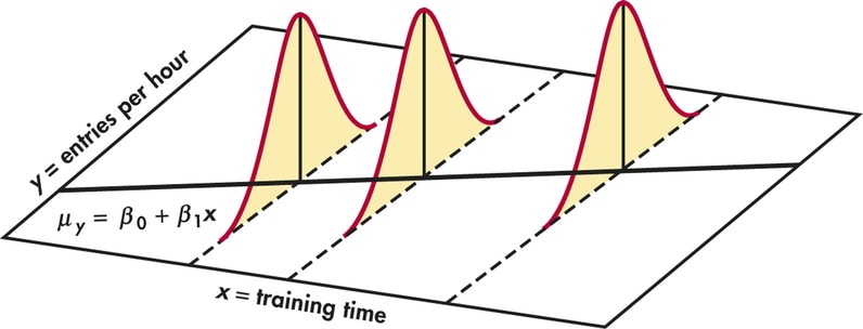
In order to perform inference in the linear regression model a further hypothesis is needed to specify the distribution of $\mathbf{y}$ conditional upon $\mathbf{X}$ :
$$
y \mid \mathbf{X} \sim \mathbf{N}\left(\mathbf{X} \boldsymbol{\beta}, \sigma^{2} I\right)
$$
or, equivalently
$$
u \mid \mathbf{X} \sim \mathbf{N}\left(\mathbf{0}, \sigma^{2} I\right)
$$
given (1.20) we can immediately derive the distribution of $(\widehat{\boldsymbol{\beta}} \mid \mathbf{X})$ which, being a linear combination of a normal distribution, is also normal:
$$
(\widehat{\boldsymbol{\beta}} \mid \mathbf{X}) \sim \mathbf{N}\left(\boldsymbol{\beta}, \sigma^{2}\left(\mathbf{X}^{\prime} \mathbf{X}\right)^{-1}\right) .
$$
(1.22) constitutes the basis to construct confidence intervals and to perform hypothesis testing in the linear regression model. Consider the following expression:
$$
\begin{aligned}
\frac{(\widehat{\boldsymbol{\beta}}-\boldsymbol{\beta})^{\prime} \mathbf{X}^{\prime} \mathbf{X}(\widehat{\boldsymbol{\beta}}-\boldsymbol{\beta})}{\sigma^{2}} &=\frac{\mathbf{u}^{\prime} \mathbf{X}\left(\mathbf{X}^{\prime} \mathbf{X}\right)^{-1} \mathbf{X}^{\prime} \mathbf{X}\left(\mathbf{X}^{\prime} \mathbf{X}\right)^{-1} \mathbf{X}^{\prime} \mathbf{u}}{\sigma^{2}} \
&=\frac{\mathbf{u}^{\prime} \mathbf{Q} \mathbf{u}}{\sigma^{2}}
\end{aligned}
$$
and, by applying the results derived in the previous section, we know that:
$$
\frac{\mathbf{u}^{\prime} \mathbf{Q u}}{\sigma^{2}} \mid \mathbf{X} \sim \chi^{2}(k)
$$
$(1.23)$ is not very useful in practice, as we do not know $\sigma^{2}$. However, we know that
$$
\frac{S(\widehat{\boldsymbol{\beta}}) \mid \mathbf{X}}{\sigma^{2}}=\frac{\mathbf{u}^{\prime} \mathbf{M u}}{\sigma^{2}} \mid \mathbf{X} \sim \chi^{2}(T-k) .
$$
经济代写|宏观经济学作业代写Macroeconomics代考|Testing the significance of subset of coefficients
In the general framework to test linear restrictions set $\mathbf{r}=0, \mathbf{R}=\left[I_{r} 0\right]$, and partition in a corresponding way $\beta$ into $\left[\beta_{1} \beta_{2}\right]$. In this case the restrictions $\mathbf{R} \beta-\mathbf{r}=0$ are equivalent to $\beta_{1}=0$ in the partitioned regression model:
$$
\mathbf{y}=\mathbf{X}{1} \beta{1}+\mathbf{X}{2} \beta{2}+\mathbf{u}
$$
in which partitioning creates two blocks of dimension $r$ and $k-r$.
Before proceeding to the discussion of hypothesis testing it useful to derive the formula for the OLS estimator in the partitioned regression model. To obtain such results partition as follows the “normal equations” $\mathbf{X}^{\prime} \mathbf{X} \widehat{\boldsymbol{\beta}}=\mathbf{X}^{\prime} \mathbf{y}$ :
$$
\left(\begin{array}{l}
\mathbf{X}{1}^{\prime} \ \mathbf{X}{2}^{\prime}
\end{array}\right)\left(\begin{array}{ll}
\mathbf{X}{1} & \mathbf{X}{2}
\end{array}\right)\left(\begin{array}{l}
\widehat{\boldsymbol{\beta}}{1} \ \widehat{\boldsymbol{\beta}}{2}
\end{array}\right)=\left(\begin{array}{l}
\mathbf{X}{1}^{\prime} \ \mathbf{X}{2}^{\prime}
\end{array}\right) \mathbf{y}
$$
or, equivalently
system (1.28) can be resolved in two stages by deriving first an expression $\widehat{\boldsymbol{\beta}}{2}$ as follows: $$ \widehat{\boldsymbol{\beta}}{2}=\left(\mathbf{X}{2}^{\prime} \mathbf{X}{2}\right)^{-1}\left(\mathbf{X}{2}^{\prime} \mathbf{y}-\mathbf{X}{2}^{\prime} \mathbf{X}{1} \widehat{\boldsymbol{\beta}}{1}\right)
$$
and then by substituting it in the first equation of $(1.28)$ to obtain:
$$
\mathbf{X}{1}^{\prime} \mathbf{X}{1} \widehat{\boldsymbol{\beta}}{1}+\mathbf{X}{1}^{\prime} \mathbf{X}{2}\left(\mathbf{X}{2}^{\prime} \mathbf{X}{2}\right)^{-1}\left(\mathbf{X}{2}^{\prime} \mathbf{y}-\mathbf{X}{2}^{\prime} \mathbf{X}{1} \widehat{\boldsymbol{\beta}}{1}\right)=\mathbf{X}{1}^{\prime} \mathbf{y}
$$
from which we have ${ }^{2}$ :
$$
\begin{aligned}
\widehat{\boldsymbol{\beta}}{1} &=\left(\mathbf{X}{1}^{\prime} \mathbf{M}{2} \mathbf{X}{1}\right)^{-1} \mathbf{X}{1}^{\prime} \mathbf{M}{2} \mathbf{y} \
\mathbf{M}{2} &=\left(\mathbf{I}-\mathbf{X}{2}\left(\mathbf{X}{2}^{\prime} \mathbf{X}{2}\right)^{-1} \mathbf{X}{2}^{\prime}\right) . \end{aligned} $$ Note that, as $\mathbf{M}{2}$ is idempotent, we can also write:
$$
\widehat{\boldsymbol{\beta}}{1}=\left(\mathbf{X}{1}^{\prime} \mathbf{M}{2}^{\prime} \mathbf{M}{2} \mathbf{X}{1}\right)^{-1} \mathbf{X}{1}^{\prime} \mathbf{M}{2}^{\prime} \mathbf{M}{2} \mathbf{y}
$$
and $\widehat{\boldsymbol{\beta}}{1}$ can be interpreted as the vector of OLS coefficients of the regression of $\mathbf{y}$ on the matrix of residuals of the regression of $\mathbf{X}{1}$ on $\mathbf{X}_{2}$. So an OLS regression on two regressors is equivalent to two OLS regressions on a single regressor (Frisch-Waugh theorem).
宏观经济学代写
经济代写|宏观经济学作业代写MACROECONOMICS代考|INFERENCE IN THE LINEAR REGRESSION MODEL
为了在线性回归模型中进行推理,需要进一步假设来指定是有条件的X:
是∣X∼ñ(Xb,σ2一世)
或者,等效地
在∣X∼ñ(0,σ2一世)
给定1.20我们可以立即得出分布(b^∣X)其中,作为正态分布的线性组合,也是正态的:
(b^∣X)∼ñ(b,σ2(X′X)−1).
1.22构成了在线性回归模型中构建置信区间和进行假设检验的基础。考虑以下表达式:
(b^−b)′X′X(b^−b)σ2=在′X(X′X)−1X′X(X′X)−1X′在σ2 =在′问在σ2
并且,通过应用上一节中得出的结果,我们知道:
在′问在σ2∣X∼χ2(ķ)
(1.23)在实践中不是很有用,因为我们不知道σ2. 然而,我们知道
小号(b^)∣Xσ2=在′米在σ2∣X∼χ2(吨−ķ).
经济代写|宏观经济学作业代写MACROECONOMICS代考|TESTING THE SIGNIFICANCE OF SUBSET OF COEFFICIENTS
在一般框架中测试线性限制集r=0,R=[一世r0], 并以相应的方式进行分区b进入[b1b2]. 在这种情况下,限制Rb−r=0相当于b1=0在分区回归模型中:
$$
\mathbf{y}=\mathbf{X}{1} \beta{1}+\mathbf{X}{2} \beta{2}+\mathbf{u}
$$
in which partitioning creates two blocks of dimension $r$ and $k-r$.
Before proceeding to the discussion of hypothesis testing it useful to derive the formula for the OLS estimator in the partitioned regression model. To obtain such results partition as follows the “normal equations” $\mathbf{X}^{\prime} \mathbf{X} \widehat{\boldsymbol{\beta}}=\mathbf{X}^{\prime} \mathbf{y}$ :
$$
\left(\begin{array}{l}
\mathbf{X}{1}^{\prime} \ \mathbf{X}{2}^{\prime}
\end{array}\right)\left(\begin{array}{ll}
\mathbf{X}{1} & \mathbf{X}{2}
\end{array}\right)\left(\begin{array}{l}
\widehat{\boldsymbol{\beta}}{1} \ \widehat{\boldsymbol{\beta}}{2}
\end{array}\right)=\left(\begin{array}{l}
\mathbf{X}{1}^{\prime} \ \mathbf{X}{2}^{\prime}
\end{array}\right) \mathbf{y}
$$
or, equivalently
system (1.28) can be resolved in two stages by deriving first an expression $\widehat{\boldsymbol{\beta}}{2}$ as follows: $$ \widehat{\boldsymbol{\beta}}{2}=\left(\mathbf{X}{2}^{\prime} \mathbf{X}{2}\right)^{-1}\left(\mathbf{X}{2}^{\prime} \mathbf{y}-\mathbf{X}{2}^{\prime} \mathbf{X}{1} \widehat{\boldsymbol{\beta}}{1}\right)
$$
然后代入第一个方程(1.28)获得:
$$
\mathbf{X}{1}^{\prime} \mathbf{X}{1} \widehat{\boldsymbol{\beta}}{1}+\mathbf{X}{1}^{\prime} \mathbf{X}{2}\left(\mathbf{X}{2}^{\prime} \mathbf{X}{2}\right)^{-1}\left(\mathbf{X}{2}^{\prime} \mathbf{y}-\mathbf{X}{2}^{\prime} \mathbf{X}{1} \widehat{\boldsymbol{\beta}}{1}\right)=\mathbf{X}{1}^{\prime} \mathbf{y}
$$
from which we have ${ }^{2}$ :
$$
\begin{aligned}
\widehat{\boldsymbol{\beta}}{1} &=\left(\mathbf{X}{1}^{\prime} \mathbf{M}{2} \mathbf{X}{1}\right)^{-1} \mathbf{X}{1}^{\prime} \mathbf{M}{2} \mathbf{y} \
\mathbf{M}{2} &=\left(\mathbf{I}-\mathbf{X}{2}\left(\mathbf{X}{2}^{\prime} \mathbf{X}{2}\right)^{-1} \mathbf{X}{2}^{\prime}\right) . \end{aligned} $$ Note that, as $\mathbf{M}{2}$ is idempotent, we can also write:
$$
\widehat{\boldsymbol{\beta}}{1}=\left(\mathbf{X}{1}^{\prime} \mathbf{M}{2}^{\prime} \mathbf{M}{2} \mathbf{X}{1}\right)^{-1} \mathbf{X}{1}^{\prime} \mathbf{M}{2}^{\prime} \mathbf{M}{2} \mathbf{y}
$$
and $\widehat{\boldsymbol{\beta}}{1}$ can be interpreted as the vector of OLS coefficients of the regression of $\mathbf{y}$ on the matrix of residuals of the regression of $\mathbf{X}{1}$ on $\mathbf{X}_{2}$. So an OLS regression on two regressors is equivalent to two OLS regressions on a single regressor (Frisch-Waugh theorem).

经经济代写|宏观经济学作业代写Macroeconomics代考 请认准UprivateTA™. UprivateTA™为您的留学生涯保驾护航。