如果你也在 怎样代写数值分析numerical analysis这个学科遇到相关的难题,请随时右上角联系我们的24/7代写客服。数值分析numerical analysis是研究使用数值逼近(相对于符号操作)来解决数学分析问题的算法(有别于离散数学)。数值分析在工程和物理科学的所有领域都有应用,在21世纪还包括生命科学和社会科学、医学、商业甚至艺术领域。
数值分析numerical analysis目前计算能力的增长使得更复杂的数值分析得以使用,在科学和工程中提供详细和现实的数学模型。数值分析的例子包括:天体力学中的常微分方程(预测行星、恒星和星系的运动),数据分析中的数值线性代数,以及用于模拟医学和生物学中活细胞的随机微分方程和马尔科夫链。
my-assignmentexpert™ 数值分析numerical analysis作业代写,免费提交作业要求, 满意后付款,成绩80\%以下全额退款,安全省心无顾虑。专业硕 博写手团队,所有订单可靠准时,保证 100% 原创。my-assignmentexpert™, 最高质量的数值分析numerical analysis作业代写,服务覆盖北美、欧洲、澳洲等 国家。 在代写价格方面,考虑到同学们的经济条件,在保障代写质量的前提下,我们为客户提供最合理的价格。 由于统计Statistics作业种类很多,同时其中的大部分作业在字数上都没有具体要求,因此数值分析numerical analysis作业代写的价格不固定。通常在经济学专家查看完作业要求之后会给出报价。作业难度和截止日期对价格也有很大的影响。
想知道您作业确定的价格吗? 免费下单以相关学科的专家能了解具体的要求之后在1-3个小时就提出价格。专家的 报价比上列的价格能便宜好几倍。
my-assignmentexpert™ 为您的留学生涯保驾护航 在数学Mathematics作业代写方面已经树立了自己的口碑, 保证靠谱, 高质且原创的数值分析numerical anaysis代写服务。我们的专家在数学Mathematics代写方面经验极为丰富,各种数值分析numerical analysis相关的作业也就用不着 说。
我们提供的数值分析numerical analysis及其相关学科的代写,服务范围广, 其中包括但不限于:

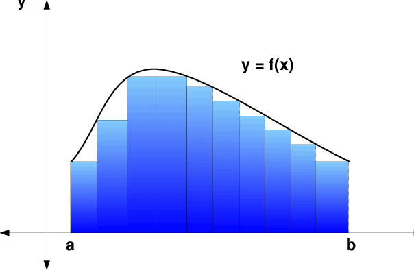
数学代写|数值分析代写numerical analysis代考|A REVIEW OF THE DEFINITE INTEGRAL
To construct the definite integral of a function, we first define the mesh points (or grid points) $x_{i}^{(n)}$ according to
$$
a=x_{0}^{(n)}<x_{1}^{(n)}<x_{2}^{(n)} \cdots<x_{n-1}^{(n)}<x_{n}^{(n)}=b
$$
and the evaluation points $\eta_{i}$ are then each taken from within the appropriate subinterval, i.e., $\eta_{i} \in\left[x_{i-1}, x_{i}\right], 1 \leq i \leq n$, arbitrarily. Now, if we assume that
$$
\lim {n \rightarrow \infty}\left[\max {1 \leq i \leq n}\left(x_{i}^{(n)}-x_{i-1}^{(n)}\right)\right]=0
$$
(this simply means that the largest distance between adjacent points goes to zero as we take more and more points), then, under very mild conditions on $f$, it can be shown that the limit
$$
L=\lim {n \rightarrow \infty} \sum{i=1}^{n} f\left(\eta_{i}\right)\left(x_{i}^{(n)}-x_{i-1}^{(n)}\right)
$$
exists and that its value is independent of the choices made for the mesh points $\left{x_{i}^{(n)}\right}$ and evaluation points $\left{\eta_{i}\right}$. When this happens, we call this limit value the definite integral of $f$, and we write
$$
L=I(f)=\int_{a}^{b} f(x) d x .
$$
Note that this construction of the integral requires very little. We only need the fact that $f$ is continuous, that the sequence of meshes is such that the distance between adjacent points becomes arbitrarily small, and that the evaluation points are taken from anywhere in each subinterval. A summation of the form
$$
R_{n}(f)=\sum_{i=1}^{n} f\left(\eta_{i}\right)\left(x_{i}^{(n)}-x_{i-1}^{(n)}\right)
$$
数学代写|数值分析代写numerical analysis代考|IMPROVING THE TRAPEZOID RULE
In $\S 2.5$ we introduced the trapezoid rule for computing integrals. Recall that, for equally spaced points, the approximation takes the form
$$
T_{n}(f)=\frac{h}{2}\left(f\left(x_{0}\right)+2 f\left(x_{1}\right)+\cdots+2 f\left(x_{n-1}\right)+f\left(x_{n}\right)\right)
$$
and the error is given by
$$
I(f)-T_{n}(f)=-\frac{b-a}{12} h^{2} f^{\prime \prime}\left(\xi_{h}\right)
$$
where $\xi_{h}$ is some value in the interval $[a, b]$.
We can improve the trapezoid rule by some deft analysis of the second derivative term in the error. Let us return to the error estimate (5.1), which we can write in the form
$$
I(f)-T_{n}(f)=-\frac{1}{12} h^{3} \sum_{i=1}^{n} f^{\prime \prime}\left(\xi_{i, h}\right)
$$
Now let’s look at the summation term, carefully. We have
$$
h^{3} \sum_{i=1}^{n} f^{\prime \prime}\left(\xi_{i, h}\right)=h^{2} \sum_{i=1}^{n} h f^{\prime \prime}\left(\xi_{i, h}\right)
$$
and the sum can be interpreted as a Riemann sum for the integral
$$
I\left(f^{\prime \prime}\right)=\int_{a}^{b} f^{\prime \prime}(x) d x=f^{\prime}(b)-f^{\prime}(a) .
$$
Thus, we know that
$$
\lim {n \rightarrow \infty} \sum{i=1}^{n} h f^{\prime \prime}\left(\xi_{i, h}\right)=f^{\prime}(b)-f^{\prime}(a)
$$
so that
$$
\sum_{i=1}^{n} h f^{\prime \prime}\left(\xi_{i, h}\right) \approx f^{\prime}(b)-f^{\prime}(a)
$$
Therefore,
$$
I(f)-T_{n}(f) \approx-\frac{1}{12} h^{2}\left(f^{\prime}(b)-f^{\prime}(a)\right) .
$$
This relationship can be interpreted and used in two equally important and useful ways:
Error estimation: We can view the quantity $\hat{E}{n}(f)=-\frac{1}{12} h^{2}\left(f^{\prime}(b)-f^{\prime}(a)\right)$ as a “computable estimate of the error” and use it to predict how many points are required to obtain a given accuracy. Bear in mind that this approach does not guarantee that we will achieve the desired accuracy. Improvement of the approximation: Define the new quadrature rule, $$ T{n}^{C}(f)=T_{n}(f)-\frac{1}{12} h^{2}\left(f^{\prime}(b)-f^{\prime}(a)\right),
$$
which we will call the corrected trapezoid rule. This value will tend to be much more accurate than that obtained using the ordinary trapezoid rule and only marginally more expensive to compute.
数学代写|数值分析代写NUMERICAL ANALYSIS代考|SIMPSON’S RULE AND DEGREE OF PRECISION
Common sense, plus the results of Chapter 4 on interpolation error, lead us to think that we might be able to do better than the trapezoid rule by using a higher degree of polynomial. Simpson’s rule is nothing more than this next logical step, relying on quadratic interpolation to generate the quadrature rule. ${ }^{2}$
We follow the basic outline from our presentation for the trapezoid rule. Thus we start by approximating $I(f)$ by a single quadratic approximation. Let $p_{2}$ be the quadratic polynomial that interpolates $f$ at the three points $x_{0}=a, x_{2}=b$, and $x_{1}=c=(a+b) / 2$, the midpoint. Define the basic Simpson’s Rule, then, as
$$
S_{2}(f)=I\left(p_{2}\right)=\int_{a}^{b}\left(L_{0}(x) f(a)+L_{1}(x) f(c)+L_{2}(x) f(b)\right) d x
$$
where the Lagrange functions are here defined as
$$
L_{0}(x)=\frac{(x-c)(x-b)}{(a-c)(a-b)}, \quad L_{1}(x)=\frac{(x-a)(x-b)}{(c-a)(c-b)}, \quad L_{2}(x)=\frac{(x-a)(x-c)}{(b-a)(b-c)}
$$
Then the quadrature rule is given by
$$
S_{2}(f)=A f(a)+C f(c)+B f(b)
$$
where
$$
A=\int_{a}^{b} L_{0}(x) d x, \quad C=\int_{a}^{b} L_{1}(x) d x, \quad B=\int_{a}^{b} L_{2}(x) d x
$$
To compute these we define $h=b-c=c-a=(b-a) / 2$, so that we have
$$
A=\int_{a}^{a+2 h} L_{0}(x) d x, C=\int_{a}^{a+2 h} L_{1}(x) d x, B=\int_{a}^{a+2 h} L_{2}(x) d x
$$
数值分析代写
数学代写|数值分析代写NUMERICAL ANALYSIS代考|A REVIEW OF THE DEFINITE INTEGRAL
为了构造函数的定积分,我们首先定义网格点这rGr一世dp这一世n吨s X一世(n)根据
$$
a=x_{0}^{(n)}<x_{1}^{(n)}<x_{2}^{(n)} \cdots<x_{n-1}^{(n)}<x_{n}^{(n)}=b
$$
and the evaluation points $\eta_{i}$ are then each taken from within the appropriate subinterval, i.e., $\eta_{i} \in\left[x_{i-1}, x_{i}\right], 1 \leq i \leq n$, arbitrarily. Now, if we assume that
$$
\lim {n \rightarrow \infty}\left[\max {1 \leq i \leq n}\left(x_{i}^{(n)}-x_{i-1}^{(n)}\right)\right]=0
$$
(this simply means that the largest distance between adjacent points goes to zero as we take more and more points), then, under very mild conditions on $f$, it can be shown that the limit
$$
L=\lim {n \rightarrow \infty} \sum{i=1}^{n} f\left(\eta_{i}\right)\left(x_{i}^{(n)}-x_{i-1}^{(n)}\right)
$$
exists and that its value is independent of the choices made for the mesh points $\left{x_{i}^{(n)}\right}$ and evaluation points $\left{\eta_{i}\right}$. When this happens, we call this limit value the definite integral of $f$, and we write
$$
L=I(f)=\int_{a}^{b} f(x) d x .
$$
Note that this construction of the integral requires very little. We only need the fact that $f$ is continuous, that the sequence of meshes is such that the distance between adjacent points becomes arbitrarily small, and that the evaluation points are taken from anywhere in each subinterval. A summation of the form
$$
R_{n}(f)=\sum_{i=1}^{n} f\left(\eta_{i}\right)\left(x_{i}^{(n)}-x_{i-1}^{(n)}\right)
$$
数学代写|数值分析代写NUMERICAL ANALYSIS代考|IMPROVING THE TRAPEZOID RULE
在§§2.5我们介绍了计算积分的梯形规则。回想一下,对于等间距的点,近似值采用以下形式
吨n(F)=H2(F(X0)+2F(X1)+⋯+2F(Xn−1)+F(Xn))
错误由下式给出
一世(F)−吨n(F)=−b−一种12H2F′′(XH)
在哪里XH是区间中的某个值[一种,b].
我们可以通过对误差中的二阶导数项进行一些巧妙的分析来改进梯形规则。让我们回到误差估计5.1,我们可以写成
一世(F)−吨n(F)=−112H3∑一世=1nF′′(X一世,H)
现在让我们仔细看看求和项。我们有
H3∑一世=1nF′′(X一世,H)=H2∑一世=1nHF′′(X一世,H)
并且总和可以解释为积分的黎曼和
一世(F′′)=∫一种bF′′(X)dX=F′(b)−F′(一种).
因此,我们知道
$$
\lim {n \rightarrow \infty} \sum {i=1}^{n} hf^{\prime \prime}\left\xi_{i, h}\对\xi_{i, h}\对=f^{\素数}b-f^{\素数}一种
s这吨H一种吨
\sum_{i=1}^{n} hf^{\prime \prime}\left\xi_{i, h}\对\xi_{i, h}\对\约 f^{\素数}b-f^{\素数}一种
$$
所以,
I(f)-T_{n}(f) \approx-\frac{1}{12} h^{2}\left(f^{\prime}(b)-f^{\prime}(a)\right) .
这种关系可以用两种同样重要和有用的方式来解释和使用:
This relationship can be interpreted and used in two equally important and useful ways:
Error estimation: We can view the quantity $\hat{E}{n}(f)=-\frac{1}{12} h^{2}\left(f^{\prime}(b)-f^{\prime}(a)\right)$ as a “computable estimate of the error” and use it to predict how many points are required to obtain a given accuracy. Bear in mind that this approach does not guarantee that we will achieve the desired accuracy. Improvement of the approximation: Define the new quadrature rule, $$ T{n}^{C}(f)=T_{n}(f)-\frac{1}{12} h^{2}\left(f^{\prime}(b)-f^{\prime}(a)\right),
$$
我们称之为修正梯形规则。该值往往比使用普通梯形规则获得的值更准确,并且计算成本略高。
数学代写|数值分析代写NUMERICAL ANALYSIS代考|SIMPSON’S RULE AND DEGREE OF PRECISION
常识,再加上第 4 章关于插值误差的结果,让我们认为,通过使用更高次的多项式,我们可能会比梯形规则做得更好。辛普森规则无非就是这下一个逻辑步骤,依靠二次插值来生成正交规则。2
我们遵循梯形规则演示文稿中的基本轮廓。因此,我们从近似开始一世(F)通过单个二次近似。让p2是插值的二次多项式F在三个点X0=一种,X2=b, 和X1=C=(一种+b)/2,中点。定义基本的辛普森规则,然后,
小号2(F)=一世(p2)=∫一种b(大号0(X)F(一种)+大号1(X)F(C)+大号2(X)F(b))dX
其中拉格朗日函数在这里定义为
大号0(X)=(X−C)(X−b)(一种−C)(一种−b),大号1(X)=(X−一种)(X−b)(C−一种)(C−b),大号2(X)=(X−一种)(X−C)(b−一种)(b−C)
那么求积规则由下式给出
小号2(F)=一种F(一种)+CF(C)+乙F(b)
在哪里
一种=∫一种b大号0(X)dX,C=∫一种b大号1(X)dX,乙=∫一种b大号2(X)dX
为了计算这些,我们定义H=b−C=C−一种=(b−一种)/2,所以我们有
一种=∫一种一种+2H大号0(X)dX,C=∫一种一种+2H大号1(X)dX,乙=∫一种一种+2H大号2(X)dX

数学代写|数值分析代写numerical analysis代考 请认准UprivateTA™. UprivateTA™为您的留学生涯保驾护航。