如果你也在 怎样代写电动力学Electrodynamics这个学科遇到相关的难题,请随时右上角联系我们的24/7代写客服。电动力学Electrodynamics研究与运动中的带电体和变化的电场和磁场有关的现象;由于运动的电荷会产生磁场,所以电动力学关注磁、电磁辐射和电磁感应等效应,包括发电机和电动机等实际应用。
电动力学Electrodynamics电动力学的这一领域,通常被称为经典电动力学,是由物理学家詹姆斯-克拉克-麦克斯韦首次系统地解释的。麦克斯韦方程,一组微分方程,非常普遍地描述了这个领域的现象。最近的发展是量子电动力学,它的制定是为了解释电磁辐射与物质的相互作用,量子理论的规律适用于此。物理学家P. A. M. Dirac, W. Heisenberg, 和W. Pauli是制定量子电动力学的先驱者。当所考虑的带电粒子的速度与光速相当时,必须进行涉及相对论的修正;该理论的这个分支被称为相对论电动力学。它被应用于粒子加速器和电子管所涉及的现象,这些电子管承受着高电压和重电流。
my-assignmentexpert™ 电动力学Electrodynamics作业代写,免费提交作业要求, 满意后付款,成绩80\%以下全额退款,安全省心无顾虑。专业硕 博写手团队,所有订单可靠准时,保证 100% 原创。my-assignmentexpert™, 最高质量的电动力学Electrodynamics作业代写,服务覆盖北美、欧洲、澳洲等 国家。 在代写价格方面,考虑到同学们的经济条件,在保障代写质量的前提下,我们为客户提供最合理的价格。 由于统计Statistics作业种类很多,同时其中的大部分作业在字数上都没有具体要求,因此电动力学Electrodynamics作业代写的价格不固定。通常在经济学专家查看完作业要求之后会给出报价。作业难度和截止日期对价格也有很大的影响。
想知道您作业确定的价格吗? 免费下单以相关学科的专家能了解具体的要求之后在1-3个小时就提出价格。专家的 报价比上列的价格能便宜好几倍。
my-assignmentexpert™ 为您的留学生涯保驾护航 在物理Physical作业代写方面已经树立了自己的口碑, 保证靠谱, 高质且原创的物理Physical代写服务。我们的专家在电动力学Electrodynamics代写方面经验极为丰富,各种电动力学Electrodynamics相关的作业也就用不着 说。
我们提供的电动力学Electrodynamics及其相关学科的代写,服务范围广, 其中包括但不限于:
物理代写|电动力学作业代写Electrodynamics代考|Hypersurfaces in Minkowski Space-Time
In this section we introduce a few notions regarding hypersurfaces in four dimensions, which will prove useful later on.
Parameterizations of hypersurfaces. By definition a hypersurface $\Gamma$ in a fourdimensional Minkowski space-time is a subset – more precisely a submanifold of $\mathbb{R}^{4}$, of dimension three. In parametric form a hypersurface is described by four functions of three parameters
$$
y^{\mu}(\boldsymbol{\lambda})
$$
where $\boldsymbol{\lambda}$ denotes the triple $\left{\lambda^{a}\right}$, with $a=1,2,3$. Alternatively one may represent a hypersurface $\Gamma$ in implicit form in terms of a single scalar function $f(x)$, through the relation
$$
x^{\mu} \in \Gamma \quad \Leftrightarrow \quad f(x)=0 .
$$
We can step from one representation to the other by inverting, for example, the spatial coordinates $\mathbf{y}(\boldsymbol{\lambda})$ of (3.11) to determine the parameters $\boldsymbol{\lambda}$ as functions of the spatial coordinates $\mathbf{x}$, i.e. by inverting the functions $\mathbf{x}=\mathbf{y}(\boldsymbol{\lambda}) \rightarrow \boldsymbol{\lambda}(\mathbf{x})$, and by setting then
$$
f(x)=f\left(x^{0}, \mathbf{x}\right)=x^{0}-y^{0}(\boldsymbol{\lambda}(\mathbf{x}))
$$
This function satisfies, in fact, the identity
$$
f(y(\boldsymbol{\lambda}))=0
$$
物理代写|电动力学作业代写Electrodynamics代考|Relativistic Invariance
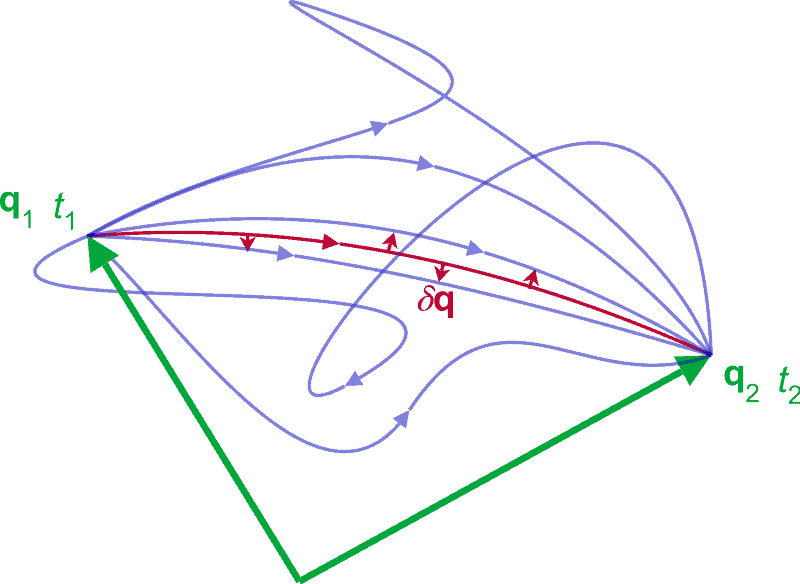
So far we have made no assumptions about the invariance properties of the considered field theory. In this section we analyze some important aspects of the principle of least action, in the particular case of a relativistic field theory.
Principle of least action and manifest covariance. As explained in Chap. 1 , in a relativistic field theory we expect the equations of motion to be manifestly covariant. In the variational framework manifest covariance is, actually, realized in a natural way, if the fields are organized into tensor multiplets, and the Lagrangian $\mathcal{L}$ is a fourscalar. In fact, in this case the Euler-Lagrange equations (3.8) are automatically manifestly covariant. In a relativistic theory we require, therefore, the Lagrangian to be invariant under the Poincaré transformations $x^{\prime}=\Lambda x+a$, more precisely we demand the equality $$
\mathcal{L}\left(\varphi^{\prime}\left(x^{\prime}\right), \partial^{\prime} \varphi^{\prime}\left(x^{\prime}\right)\right)=\mathcal{L}(\varphi(x), \partial \varphi(x))
$$
to be fulfilled for all $\Lambda_{\nu}^{\mu} \in O(1,3)$, and for all $a^{\mu}$. If this equality holds, we can ask whether the action (3.6) is a scalar, as postulated in the introduction of this chapter. Actually, from the expression (3.6) there emerges an obvious obstacle to the invariance of $I$ : whereas the measure of the integral is invariant,
$$
d^{4} x^{\prime}=|\operatorname{det} \Lambda| d^{4} x=d^{4} x
$$
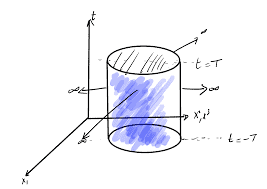
the integration domain is not, since the time variable is integrated over a finite interval. Nevertheless, it is not difficult to overcome this obstruction. In fact, it is sufficient to substitute in (3.6) the space-like hyperplanes $t=t_{1}$ and $t=t_{2}$, which bound the four-dimensional integration domain, with two generic infinitely extended and non-intersecting space-like hypersurfaces $\Gamma_{1}$ and $\Gamma_{2}$. In fact, a hyperplane at constant time is a particular space-like hypersurface, which after a Poincaré transformation is no longer a hyperplane at constant time, while remaining a space-like hypersurface. In order to overcome the above obstacle we, therefore, replace the expression (3.6) with the generalized action
$$
I[\varphi]=\int_{\Gamma_{1}}^{\Gamma_{2}} \mathcal{L}(\varphi(x), \partial \varphi(x)) d^{4} x
$$
which, thanks to the relations (3.25) and (3.26), is indeed a relativistic invariant,
$$
I^{\prime}=\int_{\Gamma_{1}^{\prime}}^{\Gamma_{2}^{\prime}} \mathcal{L}\left(\varphi^{\prime}\left(x^{\prime}\right), \partial^{\prime} \varphi^{\prime}\left(x^{\prime}\right)\right) d^{4} x^{\prime}=\int_{\Gamma_{1}}^{\Gamma_{2}} \mathcal{L}(\varphi(x), \partial \varphi(x)) d^{4} x=I
$$
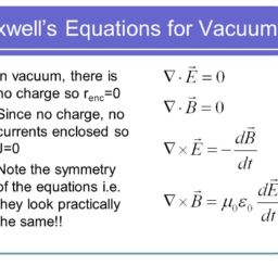
物理代写|电动力学作业代写ELECTRODYNAMICS代考|Lagrangian for Maxwell’s Equations
In this section we illustrate the variational method, retrieving the equations of the electromagnetic field through the principle of least action. In principle, our aim is thus to interpret equations (2.21) and (2.22) as the Euler-Lagrange equations relative to an appropriate Lagrangian. The first question to be addressed is the choice of the Lagrangian fields $\varphi_{r}$. Since equations (2.21) and (2.22) correspond altogether to eight equations, a priori we should hence introduce as many Lagrangian fields, namely eight. The natural choice $\varphi_{r}=F^{\mu \nu}$, which, by the way, would have the advantage of introducing only observable fields, is therefore precluded, for the Maxwell tensor corresponds not to eight, but only to six independent fields, i.e. E and $\mathbf{B}$, see in particular Problem 3.9. This strategy must hence be abandoned, and we must search for an alternative one. Such an alternative strategy consists in proceeding as anticipated in Sect. 2.2.4: we first solve the Bianchi identity in terms of a vector potential $A_{\mu}$, setting
$$
F_{\mu \nu}=\partial_{\mu} A_{\nu}-\partial_{\nu} A_{\mu}
$$
and then choose as Lagrangian fields the four components of this potential
$$
\varphi_{r}=A_{\mu}
$$
with the identification $r=\mu=0,1,2,3$. According to this approach the principle of least action should give rise to the Maxwell equation
$$
\partial_{\mu} F^{\mu \nu}-j^{\nu}=0
$$
电动力学代写
物理代写|电动力学作业代写ELECTRODYNAMICS代考|HYPERSURFACES IN MINKOWSKI SPACE-TIME
在本节中,我们将介绍一些关于四个维度的超曲面的概念,这些概念将在稍后证明是有用的。
超曲面的参数化。根据定义,超曲面Γ在四维闵可夫斯基时空是一个子集——更准确地说是R4,维度三。在参数形式中,超曲面由三个参数的四个函数描述
$$
y^{\mu}(\boldsymbol{\lambda})
$$
在哪里λ表示三元组\left{\lambda^{a}\right}\left{\lambda^{a}\right}, 和一种=1,2,3. 或者,一个可以代表超曲面Γ以单个标量函数的隐式形式F(X),通过关系
Xμ∈Γ⇔F(X)=0.
例如,我们可以通过反转空间坐标来从一种表示形式过渡到另一种表示形式是(λ)的3.11确定参数λ作为空间坐标的函数X,即通过反转函数X=是(λ)→λ(X),然后通过设置
$$
f(x)=f\left(x^{0}, \mathbf{x}\right)=x^{0}-y^{0}(\boldsymbol{\lambda}(\mathbf{x}))
$$
这个函数,其实就是满足恒等式
$$
f(y(\boldsymbol{\lambda}))=0
$$
物理代写|电动力学作业代写ELECTRODYNAMICS代考|RELATIVISTIC INVARIANCE
到目前为止,我们还没有对所考虑的场论的不变性做出任何假设。在本节中,我们分析了最小作用原理的一些重要方面,在相对论场论的特定情况下。
最小作用原则和明显协变。如第 1 章所述。如图1所示,在相对论场论中,我们期望运动方程明显是协变的。在变分框架中,如果场被组织成张量多重态,并且拉格朗日方程,则实际上以一种自然的方式实现了明显的协方差。大号是一个四标量。事实上,在这种情况下,欧拉-拉格朗日方程3.8是自动明显协变的。因此,在相对论中,我们要求拉格朗日在庞加莱变换下是不变的X′=ΛX+一种,更准确地说,我们要求平等大号(披′(X′),∂′披′(X′))=大号(披(X),∂披(X))
为所有人实现Λνμ∈这(1,3), 对于所有人一种μ. 如果这个等式成立,我们可以问这个动作是否3.6是一个标量,正如本章介绍中所假设的。其实从表达式3.6出现了一个明显的障碍一世:而积分的度量是不变的,
d4X′=|这Λ|d4X=d4X
积分域不是,因为时间变量是在有限区间内积分的。然而,要克服这个障碍并不难。事实上,替换就足够了3.6类空间超平面吨=吨1和吨=吨2,它限制了四维积分域,具有两个通用的无限扩展且不相交的类空间超曲面Γ1和Γ2. 事实上,恒定时间超平面是一个特定的类空间超曲面,经过庞加莱变换后不再是恒定时间超平面,而仍然是类空间超曲面。因此,为了克服上述障碍,我们将表达式替换为3.6用广义的动作
$$
I[\varphi]=\int_{\Gamma_{1}}^{\Gamma_{2}} \mathcal{L}(\varphi(x), \partial \varphi(x)) d^{4} x
$$
which, thanks to the relations (3.25) and (3.26), is indeed a relativistic invariant,
$$
I^{\prime}=\int_{\Gamma_{1}^{\prime}}^{\Gamma_{2}^{\prime}} \mathcal{L}\left(\varphi^{\prime}\left(x^{\prime}\right), \partial^{\prime} \varphi^{\prime}\left(x^{\prime}\right)\right) d^{4} x^{\prime}=\int_{\Gamma_{1}}^{\Gamma_{2}} \mathcal{L}(\varphi(x), \partial \varphi(x)) d^{4} x=I
$$
物理代写|电动力学作业代写ELECTRODYNAMICS代考|LAGRANGIAN FOR MAXWELL’S EQUATIONS
在本节中,我们说明变分法,通过最小作用原理检索电磁场方程。原则上,我们的目标是解释方程2.21和2.22作为相对于适当的拉格朗日方程的欧拉-拉格朗日方程。首先要解决的问题是拉格朗日场的选择披r. 由于方程2.21和2.22总共对应于八个方程,因此我们应该先验地引入尽可能多的拉格朗日场,即八个。自然的选择披r=Fμν,顺便说一下,它的优点是只引入可观察的场,因此被排除在外,因为麦克斯韦张量不对应于八个,而只对应于六个独立的场,即 E 和乙,具体见习题 3.9。因此必须放弃这种策略,我们必须寻找替代策略。这种替代策略包括按照 Sect 中的预期进行。2.2.4:我们首先根据向量势求解 Bianchi 恒等式一种μ, 环境
$$
F_{\mu \nu}=\partial_{\mu} A_{\nu}-\partial_{\nu} A_{\mu}
$$
然后选择这个势的四个分量作为拉格朗日场
$$
\varphi_{r}=A_{\mu}
$$
与身份证r=μ=0,1,2,3. 根据这种方法,最小作用原理应该产生麦克斯韦方程
$$
\partial_{\mu} F^{\mu \nu}-j^{\nu}=0
$$

物理代写|电动力学作业代写Electrodynamics代考 请认准UprivateTA™. UprivateTA™为您的留学生涯保驾护航。
电磁学代考
物理代考服务:
物理Physics考试代考、留学生物理online exam代考、电磁学代考、热力学代考、相对论代考、电动力学代考、电磁学代考、分析力学代考、澳洲物理代考、北美物理考试代考、美国留学生物理final exam代考、加拿大物理midterm代考、澳洲物理online exam代考、英国物理online quiz代考等。
光学代考
光学(Optics),是物理学的分支,主要是研究光的现象、性质与应用,包括光与物质之间的相互作用、光学仪器的制作。光学通常研究红外线、紫外线及可见光的物理行为。因为光是电磁波,其它形式的电磁辐射,例如X射线、微波、电磁辐射及无线电波等等也具有类似光的特性。
大多数常见的光学现象都可以用经典电动力学理论来说明。但是,通常这全套理论很难实际应用,必需先假定简单模型。几何光学的模型最为容易使用。
相对论代考
上至高压线,下至发电机,只要用到电的地方就有相对论效应存在!相对论是关于时空和引力的理论,主要由爱因斯坦创立,相对论的提出给物理学带来了革命性的变化,被誉为现代物理性最伟大的基础理论。
流体力学代考
流体力学是力学的一个分支。 主要研究在各种力的作用下流体本身的状态,以及流体和固体壁面、流体和流体之间、流体与其他运动形态之间的相互作用的力学分支。
随机过程代写
随机过程,是依赖于参数的一组随机变量的全体,参数通常是时间。 随机变量是随机现象的数量表现,其取值随着偶然因素的影响而改变。 例如,某商店在从时间t0到时间tK这段时间内接待顾客的人数,就是依赖于时间t的一组随机变量,即随机过程
Matlab代写
MATLAB 是一种用于技术计算的高性能语言。它将计算、可视化和编程集成在一个易于使用的环境中,其中问题和解决方案以熟悉的数学符号表示。典型用途包括:数学和计算算法开发建模、仿真和原型制作数据分析、探索和可视化科学和工程图形应用程序开发,包括图形用户界面构建MATLAB 是一个交互式系统,其基本数据元素是一个不需要维度的数组。这使您可以解决许多技术计算问题,尤其是那些具有矩阵和向量公式的问题,而只需用 C 或 Fortran 等标量非交互式语言编写程序所需的时间的一小部分。MATLAB 名称代表矩阵实验室。MATLAB 最初的编写目的是提供对由 LINPACK 和 EISPACK 项目开发的矩阵软件的轻松访问,这两个项目共同代表了矩阵计算软件的最新技术。MATLAB 经过多年的发展,得到了许多用户的投入。在大学环境中,它是数学、工程和科学入门和高级课程的标准教学工具。在工业领域,MATLAB 是高效研究、开发和分析的首选工具。MATLAB 具有一系列称为工具箱的特定于应用程序的解决方案。对于大多数 MATLAB 用户来说非常重要,工具箱允许您学习和应用专业技术。工具箱是 MATLAB 函数(M 文件)的综合集合,可扩展 MATLAB 环境以解决特定类别的问题。可用工具箱的领域包括信号处理、控制系统、神经网络、模糊逻辑、小波、仿真等。