如果你也在 怎样代写数据可视化Intro to Data Analytics & Visualization这个学科遇到相关的难题,请随时右上角联系我们的24/7代写客服。数据可视化Intro to Data Analytics & Visualization数据可视化是以图画或图形的形式表示信息和数据(例如:图表、图形和地图)。数据可视化工具提供了一种方便的方式来查看和理解数据中的趋势、模式和异常值。数据可视化工具和技术对于分析海量信息和做出数据驱动的决策至关重要。使用图片来理解数据的概念自几个世纪以来一直被使用。数据可视化的一般类型是图表、表格、图形、地图、仪表盘。
数据可视化Intro to Data Analytics & Visualization析是分析数据集的过程,以便对他们所拥有的信息做出决策,越来越多地使用专门的软件和系统。数据分析技术被用于商业行业,使组织能够做出商业决策。数据可以帮助企业更好地了解他们的客户,改善他们的广告活动,个性化他们的内容,并提高他们的底线。数据分析的技术和过程已经被自动化为机械过程和算法,在原始数据上工作,供人使用。数据分析帮助企业优化其业绩。
my-assignmentexpert™ 数据可视化Intro to Data Analytics & Visualization作业代写,免费提交作业要求, 满意后付款,成绩80\%以下全额退款,安全省心无顾虑。专业硕 博写手团队,所有订单可靠准时,保证 100% 原创。my-assignmentexpert™, 最高质量的数据可视化Intro to Data Analytics & Visualization作业代写,服务覆盖北美、欧洲、澳洲等 国家。 在代写价格方面,考虑到同学们的经济条件,在保障代写质量的前提下,我们为客户提供最合理的价格。 由于统计Statistics作业种类很多,同时其中的大部分作业在字数上都没有具体要求,因此数据可视化Intro to Data Analytics & Visualization作业代写的价格不固定。通常在经济学专家查看完作业要求之后会给出报价。作业难度和截止日期对价格也有很大的影响。
想知道您作业确定的价格吗? 免费下单以相关学科的专家能了解具体的要求之后在1-3个小时就提出价格。专家的 报价比上列的价格能便宜好几倍。
my-assignmentexpert™ 为您的留学生涯保驾护航 在data analysis作业代写方面已经树立了自己的口碑, 保证靠谱, 高质且原创的data analysis代写服务。我们的专家在数据可视化Intro to Data Analytics & Visualization代写方面经验极为丰富,各种数据可视化Intro to Data Analytics & Visualization相关的作业也就用不着 说。
我们提供的数据可视化Intro to Data Analytics & Visualization及其相关学科的代写,服务范围广, 其中包括但不限于:
data analysis代写|数据可视化代写Intro to Data Analytics & Visualization代考|Working with k-NN in R
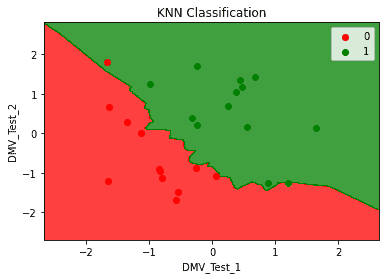
When explaining the way k-NN works, we have used the same data as training and testing data. The risk here is overfitting: there is noise in the data almost always (for instance due to measurement errors) and testing on the same dataset does not let us examine the impact of noise on our classification. In other words, we want to ensure that our classification reflects real associations in the data.
There are several ways to solve this issue. The most simple is to use a different set of data for training and testing. We have already seen this when discussing Naïve Bayes. Another, better, solution is to use cross-validation. In cross-validation, the data is split in any number of parts lower than the number of observations. One part is then left out for testing and the rest is used for training. Training is then performed again, leaving another part of the data out for testing, but including the part that was previously used for testing. We will discuss cross-validation in more detail in Chapter 14, Cross-validation and Bootstrapping Using Caret and Exporting Predictive Models Using PMML.
Here, we will use a special case of cross-validation: leave-one-out cross-validation, as this is readily implemented in the function knn. cv (), which is also included in the class package. In leave-one-out cross-validation, each observation is iteratively left out for testing, and all other observations are used for training.
data analysis代写|数据可视化代写Intro to Data Analytics & Visualization代考|Computing the performance of classification
There are several measures of performance that we can compute from the preceding table:
- The true positive rate (or sensitivity) is computed as the number of true positives divided by the number of true positives plus the number of false negatives. In our example, sensitivity is the probability that a survivor is classified as such. Sensitivity in this case is:
$$
168 /(168+186)=0.4745763
$$ - The true negative rate (or specificity) is computed as the number of true negatives divided by the number of true negatives plus the number of false positives. In our example, specificity is the probability that a nonsurvivor is classified as such. Specificity in this case is:
$$
645 /(645+60)=0.9148936
$$ - The positive predictive value (or precision) is computed as the number of true positives divided by the number of true positives plus the number of false positives. In our example, precision is the probability that individuals classified as survivors are actually survivors. Precision in this case is:
$$
168 /(168+60)=0.7368421
$$ - The negative predictive value is computed as the number of true negatives divided by the number of true negative plus the number of false negatives. In our example, the negative predictive value is the probability that individuals classified as nonsurvivors are actually nonsurvivors. In this case, its value is: $645 /(645+186)=0.7761733$
- The accuracy is computed as the number of correctly classified instances (true positives plus true negatives) divided by the number of cases correctly classified plus the number of incorrectly classified instances. In our example, accuracy is the number of survivors and nonsurvivors correctly classified as such. In this case, accuracy is:
$$
(645+168) /((645+168)+(60+186))=0.7677054
$$ - Cohen’s kappa is a measure that can be used to assess the performance of classification. Its advantage is that it adjusts for correct classification happening by chance. Its drawback is that it is slightly more complex to compute. Considering two possible class values, let’s call them No and Yes. The kappa coefficient is computed as the accuracy minus the probability of correct classification by chance, divided by 1 minus the probability of correct classification by chance. The probability of correct classification by chance is the probability of correct classification of “Yes” by chance plus the probability of correct classification of “No” by chance. The probability of the correct classification of “Yes” by chance can be computed as the probability of observed “Yes” multiplied by the probability of classified “Yes”. Likewise, the probability of correct classification of “No” by chance can be computed as the probability of observed “No” multiplied by the probability of classified “No”. Let’s compute the kappa for the preceding example.
- In the preceding example, the probability of the observed “No” is (645 $+60) /(647+60+186+168)=0.6644675$. The probability of the classified “No” is: $(645+186) /(645+186+60+168)=0.7847025$. The probability of correct classification of “No” by chance is therefore: $0.6644675$ * $0.7847025=0.5214093$. The probability of observed “Yes” is: $(186+168) /$ $(186+168+645+60)=0.3342776$. The probability of classified “Yes” is: $(60+186)$ $/(60+186+645+186)=0.2284123$. The probability of correct classification of “Yes” by chance is therefore: $0.3342776 * 0.2284123=0.07635312$. We can now compute the probability of correct classification by chance as: $0.5214093$ $+0.07635312=0.5977624$. We have seen that accuracy is $0.7677054$. We can compute the kappa as follows:
$$
(0.7677054-0.5977624) /(1-0.5977624)=0.4224941 \text {. }
$$
数据可视化代写
DATA ANALYSIS代写|数据可视化代写INTRO TO DATA ANALYTICS & VISUALIZATION代考|WORKING WITH K-NN IN R
在解释 k-NN 的工作方式时,我们使用了与训练和测试数据相同的数据。这里的风险是过度拟合:数据中几乎总是存在噪音F这r一世ns吨一种nC和d在和吨这米和一种s在r和米和n吨和rr这rs并且在同一数据集上进行测试并不能让我们检查噪声对我们分类的影响。换句话说,我们希望确保我们的分类反映数据中的真实关联。
有几种方法可以解决这个问题。最简单的是使用不同的数据集进行训练和测试。我们在讨论朴素贝叶斯时已经看到了这一点。另一个更好的解决方案是使用交叉验证。在交叉验证中,数据被分成任何数量少于观察数量的部分。然后将一部分用于测试,其余用于训练。然后再次执行训练,留下另一部分数据进行测试,但包括之前用于测试的部分。我们将在第 14 章中更详细地讨论交叉验证,使用插入符号进行交叉验证和引导以及使用 PMML 导出预测模型。
在这里,我们将使用交叉验证的一种特殊情况:留一法交叉验证,因为这很容易在函数 knn 中实现。简历,它也包含在类包中。在留一法交叉验证中,每个观察都被迭代地排除在测试之外,所有其他观察都用于训练。
DATA ANALYSIS代写|数据可视化代写INTRO TO DATA ANALYTICS & VISUALIZATION代考|COMPUTING THE PERFORMANCE OF CLASSIFICATION
我们可以从上表中计算出几种性能指标:
- 真阳性率这rs和ns一世吨一世在一世吨是计算为真阳性数除以真阳性数加上假阴性数。在我们的示例中,敏感性是幸存者被归类为此类的概率。这种情况下的灵敏度是:
168/(168+186)=0.4745763 - 真阴性率这rsp和C一世F一世C一世吨是计算为真阴性数除以真阴性数加上假阳性数。在我们的示例中,特异性是非幸存者被归类为此类的概率。在这种情况下的特异性是:
645/(645+60)=0.9148936 - 阳性预测值这rpr和C一世s一世这n计算为真阳性数除以真阳性数加上假阳性数。在我们的示例中,精确度是被归类为幸存者的个人实际上是幸存者的概率。这种情况下的精度是:
168/(168+60)=0.7368421 - 阴性预测值计算为真阴性数除以真阴性数加上假阴性数。在我们的示例中,负预测值是被归类为非幸存者的个人实际上是非幸存者的概率。在这种情况下,它的值为:645/(645+186)=0.7761733
- 准确度计算为正确分类实例的数量吨r在和p这s一世吨一世在和spl在s吨r在和n和G一种吨一世在和s除以正确分类的案例数加上错误分类的案例数。在我们的示例中,准确性是正确分类的幸存者和非幸存者的数量。在这种情况下,准确度为:
(645+168)/((645+168)+(60+186))=0.7677054 - Cohen 的 kappa 是一种可用于评估分类性能的度量。它的优点是它可以针对偶然发生的正确分类进行调整。它的缺点是计算起来稍微复杂一些。考虑到两个可能的类值,我们称它们为 No 和 Yes。kappa 系数的计算方法是准确度减去偶然正确分类的概率,再除以 1 减去偶然正确分类的概率。偶然正确分类的概率是偶然正确分类“是”的概率加上偶然正确分类“否”的概率。偶然正确分类“是”的概率可以计算为观察到“是”的概率乘以被分类为“是”的概率。同样地,偶然正确分类“否”的概率可以计算为观察到的“否”的概率乘以分类为“否”的概率。让我们计算前面示例的 kappa。
- 在前面的例子中,观察到“否”的概率是(645 $+60) /(647+60+186+168)=0.6644675$. The probability of the classified “No” is: $(645+186) /(645+186+60+168)=0.7847025$. The probability of correct classification of “No” by chance is therefore: $0.6644675$ * $0.7847025=0.5214093$. The probability of observed “Yes” is: $(186+168) /$ $(186+168+645+60)=0.3342776$. The probability of classified “Yes” is: $(60+186)$ $/(60+186+645+186)=0.2284123$. The probability of correct classification of “Yes” by chance is therefore: $0.3342776 * 0.2284123=0.07635312$. We can now compute the probability of correct classification by chance as: $0.5214093$ $+0.07635312=0.5977624$. We have seen that accuracy is $0.7677054$. We can compute the kappa as follows:
- $$
- (0.7677054-0.5977624) /(1-0.5977624)=0.4224941 \text {. }
- $$

data analysis代写|数据可视化代写Intro to Data Analytics & Visualization代考 请认准UprivateTA™. UprivateTA™为您的留学生涯保驾护航。
电磁学代考
物理代考服务:
物理Physics考试代考、留学生物理online exam代考、电磁学代考、热力学代考、相对论代考、电动力学代考、电磁学代考、分析力学代考、澳洲物理代考、北美物理考试代考、美国留学生物理final exam代考、加拿大物理midterm代考、澳洲物理online exam代考、英国物理online quiz代考等。
光学代考
光学(Optics),是物理学的分支,主要是研究光的现象、性质与应用,包括光与物质之间的相互作用、光学仪器的制作。光学通常研究红外线、紫外线及可见光的物理行为。因为光是电磁波,其它形式的电磁辐射,例如X射线、微波、电磁辐射及无线电波等等也具有类似光的特性。
大多数常见的光学现象都可以用经典电动力学理论来说明。但是,通常这全套理论很难实际应用,必需先假定简单模型。几何光学的模型最为容易使用。
相对论代考
上至高压线,下至发电机,只要用到电的地方就有相对论效应存在!相对论是关于时空和引力的理论,主要由爱因斯坦创立,相对论的提出给物理学带来了革命性的变化,被誉为现代物理性最伟大的基础理论。
流体力学代考
流体力学是力学的一个分支。 主要研究在各种力的作用下流体本身的状态,以及流体和固体壁面、流体和流体之间、流体与其他运动形态之间的相互作用的力学分支。
随机过程代写
随机过程,是依赖于参数的一组随机变量的全体,参数通常是时间。 随机变量是随机现象的数量表现,其取值随着偶然因素的影响而改变。 例如,某商店在从时间t0到时间tK这段时间内接待顾客的人数,就是依赖于时间t的一组随机变量,即随机过程
Matlab代写
MATLAB 是一种用于技术计算的高性能语言。它将计算、可视化和编程集成在一个易于使用的环境中,其中问题和解决方案以熟悉的数学符号表示。典型用途包括:数学和计算算法开发建模、仿真和原型制作数据分析、探索和可视化科学和工程图形应用程序开发,包括图形用户界面构建MATLAB 是一个交互式系统,其基本数据元素是一个不需要维度的数组。这使您可以解决许多技术计算问题,尤其是那些具有矩阵和向量公式的问题,而只需用 C 或 Fortran 等标量非交互式语言编写程序所需的时间的一小部分。MATLAB 名称代表矩阵实验室。MATLAB 最初的编写目的是提供对由 LINPACK 和 EISPACK 项目开发的矩阵软件的轻松访问,这两个项目共同代表了矩阵计算软件的最新技术。MATLAB 经过多年的发展,得到了许多用户的投入。在大学环境中,它是数学、工程和科学入门和高级课程的标准教学工具。在工业领域,MATLAB 是高效研究、开发和分析的首选工具。MATLAB 具有一系列称为工具箱的特定于应用程序的解决方案。对于大多数 MATLAB 用户来说非常重要,工具箱允许您学习和应用专业技术。工具箱是 MATLAB 函数(M 文件)的综合集合,可扩展 MATLAB 环境以解决特定类别的问题。可用工具箱的领域包括信号处理、控制系统、神经网络、模糊逻辑、小波、仿真等。