如果你也在 怎样代写电路设计Intro to circuit design这个学科遇到相关的难题,请随时右上角联系我们的24/7代写客服。电路设计Intro to circuit design一个简单的电路由电阻器、电容器、电感器、晶体管、二极管和集成电路组成。这些基本的电子元件是由导电线连接的。电流可以很容易地在这些导线之间流动,以便使电子元件处于工作状态。
电路设计Intro to circuit design过程从规格书开始,规格书说明了成品设计必须提供的功能,但没有指出如何实现这些功能。最初的规格书基本上是对客户希望成品电路实现的技术上的详细描述,可以包括各种电气要求,如电路将接收什么信号,必须输出什么信号,有什么电源,允许消耗多少功率。规格书还可以(通常也是如此)设定设计必须满足的一些物理参数,如尺寸、重量、防潮性、温度范围、热输出、振动容限和加速度容限等。
my-assignmentexpert™ 电路设计Intro to circuit design作业代写,免费提交作业要求, 满意后付款,成绩80\%以下全额退款,安全省心无顾虑。专业硕 博写手团队,所有订单可靠准时,保证 100% 原创。my-assignmentexpert™, 最高质量的电路设计Intro to circuit design作业代写,服务覆盖北美、欧洲、澳洲等 国家。 在代写价格方面,考虑到同学们的经济条件,在保障代写质量的前提下,我们为客户提供最合理的价格。 由于统计Statistics作业种类很多,同时其中的大部分作业在字数上都没有具体要求,因此电路设计Intro to circuit design作业代写的价格不固定。通常在经济学专家查看完作业要求之后会给出报价。作业难度和截止日期对价格也有很大的影响。
想知道您作业确定的价格吗? 免费下单以相关学科的专家能了解具体的要求之后在1-3个小时就提出价格。专家的 报价比上列的价格能便宜好几倍。
my-assignmentexpert™ 为您的留学生涯保驾护航 在电子工程Electrical Engineering作业代写方面已经树立了自己的口碑, 保证靠谱, 高质且原创的电子工程Electrical Engineering代写服务。我们的专家在电路设计Intro to circuit design代写方面经验极为丰富,各种电路设计Intro to circuit design相关的作业也就用不着 说。
我们提供的电路设计Intro to circuit design及其相关学科的代写,服务范围广, 其中包括但不限于:
电子工程代写|电路设计作业代写Intro to circuit design代考|Single-Layer Perceptron
Before entering deeper architectures, a simpler approach was evaluated with a network built with only an input layer and an output layer, called single-layer perceptron.
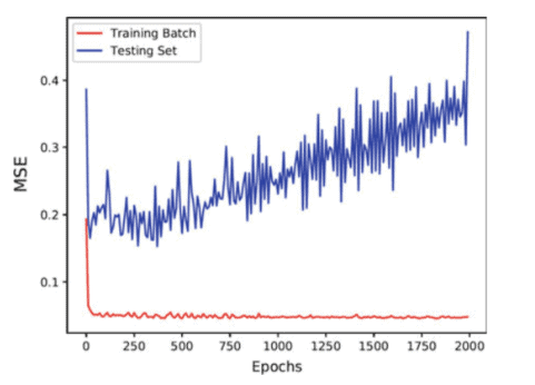
This ANN architecture represents a linear regression, where the outputs, $y$, are given by a function of an array of constants, $W$, multiplied by the input variables, $x$. The array of constants corresponds to the weights that are trained for the ANN. The first objective of this test was to evaluate if a single-layer network could present acceptable results without preprocessing the data (only scaling was applied). The results of this experiment are shown in Table $5.3$, where it is possible to observe that between 1500 and 2000 epochs the MAED on the test set starts to increase, which is a clear sign of overfitting. The linear regression model presents approximately an EOA of $60 \%$, and further developments are needed to improve this value. Nonetheless, this initial test indicates that the patterns present in the dataset can be learned by a network.
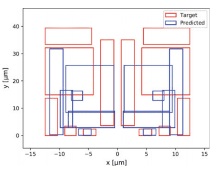
To illustrate the performance of the model, three outputs for different sizing solutions of the single-layer network trained with 2000 epochs are presented in Fig. 5.7, where (a) corresponds to the sizing with smallest MAED error, (b) to the median MAED error, and (c) to the maximum MAED error. While the worst case cannot be considered a valid placement, the median and best case are close to the target placement. For the next cases, the example with the lowest MAED is omitted, as the predicted placement solution is virtually identical to the target.
电子工程代写|电路设计作业代写Intro to circuit design代考|Multilayer Perceptron
To optimize the training time, the depth of the network is iteratively increased. If an increase in performance from a shallower to a deeper network is not significative, the increase in training time might not be justifiable to have such a deep model. The same line of thought applies to the number of units in the hidden layers. In this regard, an ANN with a single hidden layer was trained to vary the number of hidden units and the results are shown in Table 5.5. These networks took from 10 to $30 \mathrm{~min}$ to train depending on the number of hidden neurons. The performance of the ANN with one hidden layer is considerably better than the simple linear regression (single-layer perceptron), hinting that the placement problem can be better modeled by a nonlinear function. The performance of these ANNs starts to decrease when the number of hidden units is over 500 , pointing to the fact that there is no need to increase further the number of hidden units.
On the following test the depth of the network was changed to two hidden layers. These networks take $20-30 \mathrm{~min}$ to train, once again, depending on the number of hidden units, and their results are presented in Table 5.6. These networks, with two hidden layers, present better results than the ones with only one hidden layer, dropping the MAED error below $100 \mathrm{~nm}$. Since the accuracies of the networks with two hidden layers are approximately $100 \%$, it is necessary to lower the error and overlap thresholds that consider an output placement “correct”, so that if the accuracy increases in further models it is possible to weight the differences between them. By decreasing these thresholds, the accuracy will naturally decrease. These were changed to $100 \mathrm{~nm}$ and $0 \mu \mathrm{m}^{2}$, respectively, meaning only placements with no overlap are considered “correct”. The new accuracies for the two hidden layer networks are presented in Table 5.7.
Even though the thresholds for the accuracy measurment were reduced the accuracy metrics continue at high values. Meaning that the networks with two hidden layers (especially the one with 500 neurons in the first hidden layer and 250 in the second) have a high performance and output placement solutions extremely similar to the ones in the dataset. Furthermore, decreasing the overlap threshold to 0 did not have an impact on the accuracy. Since this threshold defines the border of acceptance of the placement prediction, the mean overlap area of the predicted placements that were considered being a match to their targets was actually 0 . This means that in $99.896 \%$ of the examples on the dataset, the model outputs a placement where there is no overlap at all. To further reduce the MAED error, ANNs with three hidden layers were trained. The networks took $30-40 \mathrm{~min}$ to train, and the results of these networks are presented in Table 5.8. The increase in the depth of the network did not correspond to a direct increase in the performance of the model, which may indicate that the limit to what this type of networks can learn in this specific problem.
Networks with four hidden layers were trained in an attempt to reduce the error and raise the accuracy of the models. Since these networks are deeper, they took around 50-60 min to train. The results are shown in Table 5.9. The networks with four hidden layers brought a marginal increase in the performance of the model. Specifically, there were 2 different architectures that led to better results for different reasons. The network with $1200,600,300$, and 100 hidden units in the respective hidden layers achieved a lower MAED error than the network with $1000,500,250$, and 100 hidden units, but the latter achieved a higher EA and EOA. This means that the second network has a higher mean error, but outputs placements with lower error for more examples. Therefore, this is the network architecture that will be used for further testing with four hidden layers.
For further tests of the effect of additional preprocessing methods, the network architecture that had better performance of each different number of hidden layers case study is considered. To simplify the reference to each type of network, they are henceforward designated by the names shown in Table $5.10$. The examples with the largest test error in each of the names ANNs are illustrated in Fig. 5.10. It is possible to observe that all correspond to the same sizing and that networks with 3 and 4 hidden layers are slightly closer to the target placement than the shallower networks.
电子工程代写|电路设计作业代写INTRO TO CIRCUIT DESIGN代考|Multiples Templates
To extrapolate for real-world application, the train and test sets were modified to take advantage of the different templates available on the dataset. In this first attempt, for each sizing, only the placement solution that corresponds to the placement with the smallest layout area was chosen among all the twelve templates. As some templates are better for certain devices’ sizes ranges, the dataset will contain examples with multiple conflicting guidelines spread among training and test sets. This situation makes the patterns in the data harder to learn by the algorithm. To conduct these tests, the number of epochs was increased to 1500 since the optimization algorithm takes more time to converge. A higher number of conflicting guidelines was progressively added $(2,4,8$, and finally, 12$)$, and the results are presented in Tables $5.12$ and $5.13$.
Since the existence of different conflicting guidelines in the dataset makes the patterns harder to learn, it is expected that the performance of the systems decreases significantly when comparing to the previous test cases where only one template was contemplated. ANN-3 with data centering achieves better performance in almost all tests. As the number of different templates increases, the performance of the model starts to decrease as expected, due to the variation in patterns it is trying to learn. Even though the output of the model is not optimal, it is still capable of outputting a meaningful placement as shown in Fig. 5.12. Although the overlap is high in this case, it is observable that it is trying to follow the patterns of a template, being almost completely symmetric. This fact means that the network learned the patterns of a template or subgroup of templates and applied to this example, even if not the intended originally by the test set.

电路设计作业代写
电子工程代写|电路设计作业代写INTRO TO CIRCUIT DESIGN代考|SINGLE-LAYER PERCEPTRON
在进入更深层次的架构之前,一种更简单的方法是使用仅由输入层和输出层构建的网络进行评估,称为单层感知器。
这种 ANN 架构代表一个线性回归,其中输出,是, 由常量数组的函数给出,在,乘以输入变量,X. 常量数组对应于为 ANN 训练的权重。该测试的第一个目标是评估单层网络是否可以在不预处理数据的情况下呈现可接受的结果这nl是sC一种l一世nG在一种s一种ppl一世和d. 本实验结果见表5.3,可以观察到在 1500 到 2000 个时期之间,测试集上的 MAED 开始增加,这是过度拟合的明显迹象。线性回归模型的 EOA 大约为60%,需要进一步的开发来提高这个值。尽管如此,这个初始测试表明数据集中存在的模式可以由网络学习。
为了说明模型的性能,图 5.7 显示了用 2000 个 epoch 训练的单层网络的不同尺寸解决方案的三个输出,其中一种对应于具有最小 MAED 误差的尺寸,b到中值 MAED 误差,以及C到最大 MAED 误差。虽然不能将最坏情况视为有效展示位置,但中值和最佳情况接近目标展示位置。对于接下来的情况,MAED 最低的示例被省略,因为预测的放置解决方案实际上与目标相同。
电子工程代写|电路设计作业代写INTRO TO CIRCUIT DESIGN代考|MULTILAYER PERCEPTRON
为了优化训练时间,网络的深度不断增加。如果从较浅的网络到较深的网络的性能提升并不显着,那么训练时间的增加对于拥有如此深的模型可能是不合理的。同样的思路也适用于隐藏层中的单元数量。在这方面,训练了一个具有单个隐藏层的人工神经网络来改变隐藏单元的数量,结果如表 5.5 所示。这些网络从 10 到30 米一世n根据隐藏神经元的数量进行训练。具有一个隐藏层的人工神经网络的性能明显优于简单的线性回归s一世nGl和−l一种是和rp和rC和p吨r这n,暗示放置问题可以通过非线性函数更好地建模。当隐藏单元的数量超过 500 时,这些 ANN 的性能开始下降,这表明没有必要进一步增加隐藏单元的数量。
在接下来的测试中,网络的深度被更改为两个隐藏层。这些网络采取20−30 米一世n再次根据隐藏单元的数量进行训练,其结果如表 5.6 所示。这些具有两个隐藏层的网络比只有一个隐藏层的网络呈现出更好的结果,从而降低了下面的 MAED 错误100 n米. 由于具有两个隐藏层的网络的精度大约为100%,有必要降低考虑输出放置“正确”的错误和重叠阈值,以便如果进一步模型中的准确性增加,则可以对它们之间的差异进行加权。通过降低这些阈值,准确度自然会降低。这些被改为100 n米和0μ米2,分别意味着只有没有重叠的展示位置被认为是“正确的”。两个隐藏层网络的新精度如表 5.7 所示。
即使准确度测量的阈值降低了,准确度指标仍然保持在高值。这意味着具有两个隐藏层的网络和sp和C一世一种ll是吨H和这n和在一世吨H500n和在r这ns一世n吨H和F一世rs吨H一世dd和nl一种是和r一种nd250一世n吨H和s和C这nd具有与数据集中的非常相似的高性能和输出放置解决方案。此外,将重叠阈值降低到 0 对准确性没有影响。由于此阈值定义了放置预测的接受边界,因此被认为与其目标匹配的预测放置的平均重叠区域实际上是 0 。这意味着在99.896%在数据集上的示例中,模型输出一个完全没有重叠的位置。为了进一步减少 MAED 误差,训练了具有三个隐藏层的 ANN。网络采取了30−40 米一世n进行训练,这些网络的结果如表 5.8 所示。网络深度的增加并不对应于模型性能的直接增加,这可能表明这种类型的网络在这个特定问题中可以学习的内容有限。
训练具有四个隐藏层的网络以试图减少错误并提高模型的准确性。由于这些网络更深,他们需要大约 50-60 分钟来训练。结果如表 5.9 所示。具有四个隐藏层的网络带来了模型性能的边际提升。具体来说,由于不同的原因,有两种不同的架构导致了更好的结果。网络与1200,600,300,并且各个隐藏层中的 100 个隐藏单元实现的 MAED 误差低于具有1000,500,250, 和 100 个隐藏单元,但后者实现了更高的 EA 和 EOA。这意味着第二个网络具有更高的平均误差,但输出具有更低误差的展示位置以获得更多示例。因此,这是用于进一步测试四个隐藏层的网络架构。
为了进一步测试附加预处理方法的效果,我们考虑了在每个不同数量的隐藏层案例研究中具有更好性能的网络架构。为了简化对每种类型网络的引用,因此它们由表中所示的名称指定5.10. 图 5.10 显示了每个名称 ANN 中测试误差最大的示例。可以观察到,所有这些都对应于相同的大小,并且具有 3 和 4 个隐藏层的网络比较浅的网络更接近目标位置。
电子工程代写|电路设计作业代写INTRO TO CIRCUIT DESIGN代考|MULTIPLES TEMPLATES
为了推断现实世界的应用,对训练集和测试集进行了修改,以利用数据集上可用的不同模板。在第一次尝试中,对于每种尺寸,在所有 12 个模板中仅选择与具有最小布局区域的布局相对应的布局解决方案。由于某些模板更适合某些设备的尺寸范围,因此数据集将包含分布在训练集和测试集之间的具有多个冲突准则的示例。这种情况使算法更难学习数据中的模式。为了进行这些测试,由于优化算法需要更多时间来收敛,所以 epoch 的数量增加到 1500。逐渐增加了更多相互冲突的指南(2,4,8,最后,12), 结果列于表中5.12和5.13.
由于数据集中存在不同的冲突准则使得模式更难学习,因此与之前只考虑一个模板的测试用例相比,预计系统的性能会显着下降。具有数据中心功能的 ANN-3 在几乎所有测试中都取得了更好的性能。随着不同模板数量的增加,模型的性能开始按预期下降,这是由于它试图学习的模式的变化。即使模型的输出不是最优的,它仍然能够输出一个有意义的位置,如图 5.12 所示。尽管在这种情况下重叠很高,但可以观察到它试图遵循模板的模式,几乎完全对称。

电子工程代写|电路设计作业代写Intro to circuit design代考 请认准UprivateTA™. UprivateTA™为您的留学生涯保驾护航。
电磁学代考
物理代考服务:
物理Physics考试代考、留学生物理online exam代考、电磁学代考、热力学代考、相对论代考、电动力学代考、电磁学代考、分析力学代考、澳洲物理代考、北美物理考试代考、美国留学生物理final exam代考、加拿大物理midterm代考、澳洲物理online exam代考、英国物理online quiz代考等。
光学代考
光学(Optics),是物理学的分支,主要是研究光的现象、性质与应用,包括光与物质之间的相互作用、光学仪器的制作。光学通常研究红外线、紫外线及可见光的物理行为。因为光是电磁波,其它形式的电磁辐射,例如X射线、微波、电磁辐射及无线电波等等也具有类似光的特性。
大多数常见的光学现象都可以用经典电动力学理论来说明。但是,通常这全套理论很难实际应用,必需先假定简单模型。几何光学的模型最为容易使用。
相对论代考
上至高压线,下至发电机,只要用到电的地方就有相对论效应存在!相对论是关于时空和引力的理论,主要由爱因斯坦创立,相对论的提出给物理学带来了革命性的变化,被誉为现代物理性最伟大的基础理论。
流体力学代考
流体力学是力学的一个分支。 主要研究在各种力的作用下流体本身的状态,以及流体和固体壁面、流体和流体之间、流体与其他运动形态之间的相互作用的力学分支。
随机过程代写
随机过程,是依赖于参数的一组随机变量的全体,参数通常是时间。 随机变量是随机现象的数量表现,其取值随着偶然因素的影响而改变。 例如,某商店在从时间t0到时间tK这段时间内接待顾客的人数,就是依赖于时间t的一组随机变量,即随机过程
Matlab代写
MATLAB 是一种用于技术计算的高性能语言。它将计算、可视化和编程集成在一个易于使用的环境中,其中问题和解决方案以熟悉的数学符号表示。典型用途包括:数学和计算算法开发建模、仿真和原型制作数据分析、探索和可视化科学和工程图形应用程序开发,包括图形用户界面构建MATLAB 是一个交互式系统,其基本数据元素是一个不需要维度的数组。这使您可以解决许多技术计算问题,尤其是那些具有矩阵和向量公式的问题,而只需用 C 或 Fortran 等标量非交互式语言编写程序所需的时间的一小部分。MATLAB 名称代表矩阵实验室。MATLAB 最初的编写目的是提供对由 LINPACK 和 EISPACK 项目开发的矩阵软件的轻松访问,这两个项目共同代表了矩阵计算软件的最新技术。MATLAB 经过多年的发展,得到了许多用户的投入。在大学环境中,它是数学、工程和科学入门和高级课程的标准教学工具。在工业领域,MATLAB 是高效研究、开发和分析的首选工具。MATLAB 具有一系列称为工具箱的特定于应用程序的解决方案。对于大多数 MATLAB 用户来说非常重要,工具箱允许您学习和应用专业技术。工具箱是 MATLAB 函数(M 文件)的综合集合,可扩展 MATLAB 环境以解决特定类别的问题。可用工具箱的领域包括信号处理、控制系统、神经网络、模糊逻辑、小波、仿真等。