如果你也在 怎样代写随机分析stochastic analysis MAST90059这个学科遇到相关的难题,请随时右上角联系我们的24/7代写客服。随机分析stochastic analysis或随机过程可以被定义为由一些数学集合索引的随机变量的集合,这意味着随机过程的每个随机变量都与该集合中的一个元素唯一相关。历史上,索引集是实线的某个子集,如自然数,从而使索引集有了时间的解释。集合中的每个随机变量都从同一数学空间取值,称为状态空间。
随机分析stochastic analysis在概率论和相关领域,随机(/stoʊˈkæstɪk/)或随机过程是一个数学对象,通常被定义为一个随机变量系列。随机过程被广泛用作系统和现象的数学模型,这些系统和现象似乎以随机的方式变化。这方面的例子包括细菌种群的生长,由于热噪声而波动的电流,或气体分子的运动。 随机过程在许多学科中都有应用,如生物学、化学、生态学、神经科学、物理学、 图像处理、信号处理、控制理论、信息理论、计算机科学、密码学和电信。此外,金融市场中看似随机的变化也促使随机过程在金融中得到广泛使用。
随机分析stochastic analysis代写,免费提交作业要求, 满意后付款,成绩80\%以下全额退款,安全省心无顾虑。专业硕 博写手团队,所有订单可靠准时,保证 100% 原创。最高质量的随机分析stochastic analysis作业代写,服务覆盖北美、欧洲、澳洲等 国家。 在代写价格方面,考虑到同学们的经济条件,在保障代写质量的前提下,我们为客户提供最合理的价格。 由于统计Statistics作业种类很多,同时其中的大部分作业在字数上都没有具体要求,因此随机分析stochastic analysis作业代写的价格不固定。通常在经济学专家查看完作业要求之后会给出报价。作业难度和截止日期对价格也有很大的影响。
同学们在留学期间,都对各式各样的作业考试很是头疼,如果你无从下手,不如考虑my-assignmentexpert™!
my-assignmentexpert™提供最专业的一站式服务:Essay代写,Dissertation代写,Assignment代写,Paper代写,Proposal代写,Proposal代写,Literature Review代写,Online Course,Exam代考等等。my-assignmentexpert™专注为留学生提供Essay代写服务,拥有各个专业的博硕教师团队帮您代写,免费修改及辅导,保证成果完成的效率和质量。同时有多家检测平台帐号,包括Turnitin高级账户,检测论文不会留痕,写好后检测修改,放心可靠,经得起任何考验!
想知道您作业确定的价格吗? 免费下单以相关学科的专家能了解具体的要求之后在1-3个小时就提出价格。专家的 报价比上列的价格能便宜好几倍。
我们在金融 Finaunce代写方面已经树立了自己的口碑, 保证靠谱, 高质且原创的金融 Finaunce代写服务。我们的专家在随机分析stochastic analysis代写方面经验极为丰富,各种随机分析stochastic analysis相关的作业也就用不着 说。
金融代写|随机分析代写Stochastic Analysis代考|Architectures of the deep neural networks
The change of probability detailed in Subsection $3.1$ allows us to turn the initial partial information Problem (4) into a full observation problem as
$$
\begin{aligned}
V_{0}:=\sup {\alpha \in \mathcal{A}{0}^{q}} \mathbb{E}\left[U\left(X_{N}^{\alpha}\right)\right] &=\sup {\alpha \in \mathcal{A}{0}^{q}} \overline{\mathbb{E}}\left[\bar{\Lambda}{N} U\left(X{N}^{\alpha}\right)\right] \
&=\sup {\alpha \in \mathcal{A}{0}^{q}} \overline{\mathbb{E}}\left[\overline{\mathbb{E}}\left[\bar{\Lambda}{N} U\left(X{N}^{\alpha}\right) \mid \mathcal{F}{N}^{o}\right]\right] \ &=\sup {\alpha \in \mathcal{A}{0}^{q}} \overline{\mathbb{E}}\left[U\left(X{N}^{\alpha}\right) \pi_{N}\left(\mathbb{R}^{d}\right)\right],
\end{aligned}
$$
from Bayes formula, the law of conditional expectations, and the definition of the unnormalized filter $\pi_{N}$ valued in $\mathcal{M}{+}$, the set of nonnegative measures on $\mathbb{R}^{d}$. In view of Equation (3), Proposition 1, and Proposition 2, we then introduce the dynamic value function associated to Problem (8) as $$ v{k}(x, z, \mu)=\sup {\alpha \in \mathcal{A}{k}^{q}(x, z)} J_{k}(x, z, \mu, \alpha), \quad k \in \llbracket 0, N \rrbracket,(x, z) \in \mathcal{S}^{q}, \mu \in \mathcal{M}{+}, $$ with $$ J{k}(x, z, \mu, \alpha)=\overline{\mathbb{E}}\left[U\left(X_{N}^{k, x, \alpha}\right) \pi_{N}^{k, \mu}\left(\mathbb{R}^{d}\right)\right],
$$
where $X^{k, x, \alpha}$ is the solution to Equation (3) on $\llbracket k, N \rrbracket$, starting at $X_{k}^{k, x, \alpha}=x$ at time $k$, controlled by $\alpha \in \mathcal{A}{k}^{q}(x, z)$, and $\left(\pi{\ell}^{k, \mu}\right){\ell=k, \ldots, N}$ is the solution to (6) on $\mathcal{M}{+}$, starting from $\pi_{k}^{k, \mu}=\mu$, so that $V_{0}=v_{0}\left(x_{0}, x_{0}, \mu_{0}\right)$. Here, $\mathcal{A}{k}^{q}(x, z)$ is the set of admissible investment strategies embedding the drawdown constraint: $X{\ell}^{k, x, \alpha} \geq$ $q Z_{\ell}^{k, x, z, \alpha}, \ell=k, \ldots, N$, where the maximum wealth process $Z^{k, x, z, \alpha}$ follows the dynamics: $Z_{\ell+1}^{k, x, z, \alpha}=\max \left[Z_{\ell}^{k, x, z, \alpha}, X_{\ell+1}^{k, x, \alpha}\right], \ell=k, \ldots, N-1$, starting from $Z_{k}^{k, x, z, \alpha}$ $=z$ at time $k$. The dependence of the value function upon the unnormalized filter $\mu$ means that the probability distribution on the drift is updated at each time step from Bayesian learning by observing assets price.
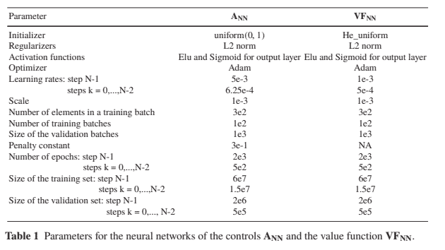
We follow the indications in [10] to setup and define the values of the various inputs of the neural networks which are listed in Table $1 .$
To train the NN, we simulate the input data. For the conditional expectation $\hat{B}{k}$, we use its time-dependent Gaussian distribution (see Remark 1): $\hat{B}{k} \sim \mathcal{N}\left(b_{0}, \Sigma_{0}-\Sigma_{k}\right)$, with $\Sigma_{k}$ as in Equation (17). On the other hand, the training of $\rho$ is drawn from the uniform distribution between $q$ and 1 , the interval where it lies according to the maximum drawdown constraint.
金融代写|随机分析代写Stochastic Analysis代考|Hybrid-Now algorithm
We use the Hybrid-Now algorithm developped in [1] in order to solve numerically our problem. This algorithm combines optimal policy estimation by neural networks and dynamic programming principle which suits the approach we have developped in Section $4 .$
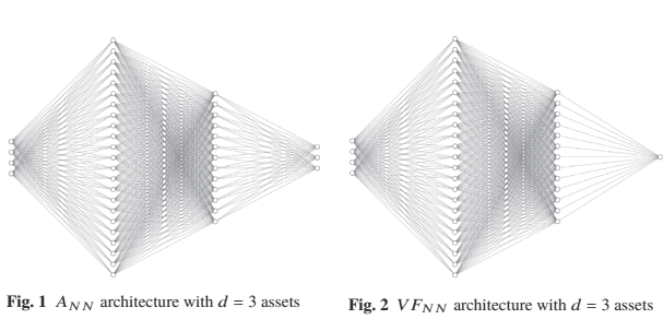
With the same notations as in Algorithm 1 detailed in the next insert, at time $k$, the algorithm computes the proxy of the optimal control $\hat{\alpha}{k}$ with $A{N N}$, using the known function $\hat{V}{k+1}$ calculated the step before, and uses $V{N N}$ to obtain a proxy of the value function $\hat{V}{k}$. Starting from the known function $\hat{V}{N}:=U$ at terminal time $N$, the algorithm computes sequentially $\hat{\alpha}{k}$ and $\hat{V}{k}$ with backward iteration until time 0 . This way, the algorithm loops to build the optimal controls and the value function pointwise and gives as output the optimal strategy, namely the optimal controls from 0 to $N-1$ and the value function at each of the $N$ time steps.
The maximum drawdown constraint is a time-dependent constraint on the maximal proportion of wealth to invest (recall Lemma 1). In practice, it is a constraint on the sum of weights of each asset or equivalently on the output of $A_{N N}$. For that reason, we have implemented an appropriate penalty function that will reject undesirable values:
$$
G_{\text {Penalty }}(A, r)=K \max \left(|A|_{1} \leq 1-\frac{q}{r}, 0\right), \quad A \in[0,1]^{d}, \quad r \in[q, 1] .
$$
随机分析代写
金融代写|随机分析代写STOCHASTIC ANALYSIS代 考|ARCHITECTURES OF THE DEEP NEURAL NETWORKS
小节中详述的概率变化 $3.1$ 允许我们把初始的部分信息问题 4 成一个完整的观㟯问题
$$
V_{0}:=\sup \alpha \in \mathcal{A} 0^{q} \mathbb{E}\left[U\left(X_{N}^{\alpha}\right)\right]=\sup \alpha \in \mathcal{A} 0^{q} \overline{\mathbb{E}}\left[\bar{\Lambda} N U\left(X N^{\alpha}\right)\right] \quad=\sup \alpha \in \mathcal{A} 0^{q} \overline{\mathbb{E}}\left[\overline{\mathbb{E}}\left[\bar{\Lambda} N U\left(X N^{\alpha}\right) \mid \mathcal{F} N^{o}\right]\right]=\sup \alpha \in \mathcal{A} 0^{q} \overline{\mathbb{E}}\left[U\left(X N^{\alpha}\right) \pi_{N}\left(\mathbb{R}^{d}\right)\right.
$$ 数8作为
$$
v k(x, z, \mu)=\sup \alpha \in \mathcal{A} k^{q}(x, z) J_{k}(x, z, \mu, \alpha), \quad k \in \backslash \text { llbracket } 0, N \backslash \operatorname{rrbracket},(x, z) \in \mathcal{S}^{q}, \mu \in \mathcal{M}+,
$$
和
$$
J k(x, z, \mu, \alpha)=\overline{\mathbb{E}}\left[U\left(X_{N}^{k, x, \alpha}\right) \pi_{N}^{k, \mu}\left(\mathbb{R}^{d}\right)\right]
$$
在哪里 $X^{k, x, \alpha}$ 是方程的解 3 上 $\backslash$ llbracket $k, N \backslash$ rrbracket,开始于 $X_{k}^{k, x, \alpha}=x$ 有时 $k$ ,受控制于 $\alpha \in \mathcal{A} k^{q}(x, z)$ ,和 $\left(\pi \ell^{k, \mu}\right) \ell=k, \ldots, N$ 是解决方䅁 6 上 $\mathcal{M}+$ , 从…开始 $\pi_{k}^{k, \mu}=\mu_{\text {, 以便 }} V_{0}=v_{0}\left(x_{0}, x_{0}, \mu_{0}\right)$. 这里, $\mathcal{A} k^{q}(x, z)$ 是嵌入回撤约束的一组可接受的投资策略: $X \ell^{k, x, \alpha} \geq q Z_{\ell}^{k, x, z, \alpha}, \ell=k, \ldots, N$ ,其中最大财富过 程 $Z^{k, x, z, z}$ 邅循动态: $Z_{\ell+1}^{k, x, z, \alpha}=\max \left[Z_{\ell}^{k, x, z, \alpha}, X_{\ell+1}^{k, x, \alpha}\right], \ell=k, \ldots, N-1$ ,从…开始 $Z_{k}^{k, x, z, \alpha}=z$ 有时 $k$. 价值函数对非归一化滤波器的依赖性 $\mu$ 意味差漂移上的概 率分布通过观崇资产价格从贝叶斯学习的每个时间步更新。
我们逼唕中的指示
10
设置和定义表中列出的神经网络的各种输入的值 1 .
isdrawn fromtheuniformdistributionbetween q\$ 和 1 ,根据最大回撤约束它所在的区间。
金融代写|随机分析代写STOCHASTIC ANALYSIS代考|HYBRIDNOW ALGORITHM
我们使用 Hybrid-Now 算法
为了在数值上解决我们的问题。该算法结合了神经网络的最优策略估计和适合我们在第 1 节中开发的方法的动态规划原理 4 .
使用与下一个揷入中详述的算法 1 中相同的符号,在时间 $k$ ,算法计算最优控制的代理 $\$$ \hat ${$ alpha} ${k h w i t h$ 一个[NN $}, u s i n g t h e k n o w n f u n c t i o n \backslash$ hat ${\mathrm{V}}$ {k+1}
ñ, thealgorithmcomputessequentially $\backslash$ hat ${\backslash$ alpha} ${k|a n d|$ hat ${V}{k}$
withbackwarditerationuntiltime0. Thisway, thealgo it
最大回撒约束是对最大财富投资比例的时间依赖性约束 recallLemma1. 在实践中,它是对每项资产权重总和或等效于 $A_{N N}$. 出于这个原因,我们已经实现了一个
远当的惩罚函数,它将拒绝不需要的值:
$$
G_{\text {Penalty }}(A, r)=K \max \left(|A|_{1} \leq 1-\frac{q}{r}, 0\right), \quad A \in[0,1]^{d}, \quad r \in[q, 1] .
$$

金融代写|随机分析代写Stochastic Analysis代考 请认准UprivateTA™. UprivateTA™为您的留学生涯保驾护航。
微观经济学代写
微观经济学是主流经济学的一个分支,研究个人和企业在做出有关稀缺资源分配的决策时的行为以及这些个人和企业之间的相互作用。my-assignmentexpert™ 为您的留学生涯保驾护航 在数学Mathematics作业代写方面已经树立了自己的口碑, 保证靠谱, 高质且原创的数学Mathematics代写服务。我们的专家在图论代写Graph Theory代写方面经验极为丰富,各种图论代写Graph Theory相关的作业也就用不着 说。
线性代数代写
线性代数是数学的一个分支,涉及线性方程,如:线性图,如:以及它们在向量空间和通过矩阵的表示。线性代数是几乎所有数学领域的核心。
博弈论代写
现代博弈论始于约翰-冯-诺伊曼(John von Neumann)提出的两人零和博弈中的混合策略均衡的观点及其证明。冯-诺依曼的原始证明使用了关于连续映射到紧凑凸集的布劳威尔定点定理,这成为博弈论和数学经济学的标准方法。在他的论文之后,1944年,他与奥斯卡-莫根斯特恩(Oskar Morgenstern)共同撰写了《游戏和经济行为理论》一书,该书考虑了几个参与者的合作游戏。这本书的第二版提供了预期效用的公理理论,使数理统计学家和经济学家能够处理不确定性下的决策。
微积分代写
微积分,最初被称为无穷小微积分或 “无穷小的微积分”,是对连续变化的数学研究,就像几何学是对形状的研究,而代数是对算术运算的概括研究一样。
它有两个主要分支,微分和积分;微分涉及瞬时变化率和曲线的斜率,而积分涉及数量的累积,以及曲线下或曲线之间的面积。这两个分支通过微积分的基本定理相互联系,它们利用了无限序列和无限级数收敛到一个明确定义的极限的基本概念 。
计量经济学代写
什么是计量经济学?
计量经济学是统计学和数学模型的定量应用,使用数据来发展理论或测试经济学中的现有假设,并根据历史数据预测未来趋势。它对现实世界的数据进行统计试验,然后将结果与被测试的理论进行比较和对比。
根据你是对测试现有理论感兴趣,还是对利用现有数据在这些观察的基础上提出新的假设感兴趣,计量经济学可以细分为两大类:理论和应用。那些经常从事这种实践的人通常被称为计量经济学家。
MATLAB代写
MATLAB 是一种用于技术计算的高性能语言。它将计算、可视化和编程集成在一个易于使用的环境中,其中问题和解决方案以熟悉的数学符号表示。典型用途包括:数学和计算算法开发建模、仿真和原型制作数据分析、探索和可视化科学和工程图形应用程序开发,包括图形用户界面构建MATLAB 是一个交互式系统,其基本数据元素是一个不需要维度的数组。这使您可以解决许多技术计算问题,尤其是那些具有矩阵和向量公式的问题,而只需用 C 或 Fortran 等标量非交互式语言编写程序所需的时间的一小部分。MATLAB 名称代表矩阵实验室。MATLAB 最初的编写目的是提供对由 LINPACK 和 EISPACK 项目开发的矩阵软件的轻松访问,这两个项目共同代表了矩阵计算软件的最新技术。MATLAB 经过多年的发展,得到了许多用户的投入。在大学环境中,它是数学、工程和科学入门和高级课程的标准教学工具。在工业领域,MATLAB 是高效研究、开发和分析的首选工具。MATLAB 具有一系列称为工具箱的特定于应用程序的解决方案。对于大多数 MATLAB 用户来说非常重要,工具箱允许您学习和应用专业技术。工具箱是 MATLAB 函数(M 文件)的综合集合,可扩展 MATLAB 环境以解决特定类别的问题。可用工具箱的领域包括信号处理、控制系统、神经网络、模糊逻辑、小波、仿真等。