MY-ASSIGNMENTEXPERT™可以为您提供 utstat.utoronto Stats531 Time series analysis时间序列分析的代写代考和辅导服务!
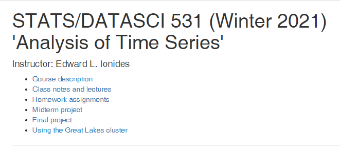
Stats531课程简介
Course description
This course gives an introduction to time series analysis using time domain methods and frequency domain methods. The goal is to acquire the theoretical and computational skills required to investigate data collected as a time series. The first half of the course will develop classical time series methodology, including auto-regressive moving average (ARMA) models, regression with ARMA errors, and estimation of the spectral density. The second half of the course will focus on state space model techniques for fitting structured dynamic models to time series data. We will progress from fitting linear, Gaussian dynamic models to fitting nonlinear models for which Monte Carlo methods are required. Examples will be drawn from ecology, economics, epidemiology, finance and elsewhere.
Prerequisites
Grading
Weekly homeworks (25%, due Tuesdays, in class).
A midterm exam (25%, in class on Thursday 2/25).
A midterm project analyzing a time series of your choice using methods covered in the first half of the course (15%, due Thursday 3/10).
A final project analyzing a time series of your choice using methods covered in the entire course (35%, due Thursday 4/28).
Discussion of homework problems is encouraged, but solutions must be written up individually. Direct copying is not acceptable.
Any material taken from any source, such as the internet, must be properly acknowledged. Unattributed copying from any source is plagiarism, and has potentially serious consequences.
Stats531 Time series analysis HELP(EXAM HELP, ONLINE TUTOR)
Question 1.1. Recall the basic properties of covariance, $\operatorname{Cov}(X, Y)=E[(X-\mathrm{E}[X])(Y-E[Y])]$, following the convention that upper case letters are random variables and lower case letters are constants:
P1. $\operatorname{Cov}(Y, Y)=\operatorname{Var}(Y)$,
P2. $\operatorname{Cov}(X, Y)=\operatorname{Cov}(Y, X)$,
P3. $\operatorname{Cov}(a X, b Y)=a b \operatorname{Cov}(X, Y)$,
P4. $\operatorname{Cov}\left(\sum_{m=1}^M Y_m, \sum_{n=1}^N Y_n\right)=\sum_{m=1}^M \sum_{n=1}^N \operatorname{Cov}\left(Y_m, Y_n\right)$.
Let $Y_{1: N}$ be a covariance stationary time series model with autocovariance function $\gamma_h$ and constant mean function, $\mu_n=\mu$. Consider the sample mean as an estimator of $\mu$,
$$
\hat{\mu}\left(y_{1: N}\right)=\frac{1}{N} \sum_{n=1}^N y_n
$$
Show how the basic properties of covariance can be used to derive the expression,
$$
\operatorname{Var}\left(\hat{\mu}\left(Y_{1: N}\right)\right)=\frac{1}{N} \gamma_0+\frac{2}{N^2} \sum_{h=1}^{N-1}(N-h) \gamma_h
$$
$\begin{aligned} \operatorname{Var}\left(\hat{\mu}\left(Y_{1: N}\right)\right) & =\operatorname{Var}\left(\frac{1}{N} \sum_{n=1}^N Y_n\right) \ & =\frac{1}{N^2} \operatorname{Cov}\left(\sum_{m=1}^N Y_m, \sum_{n=1}^N Y_n\right) \text { using } \mathrm{P} 1 \text { and } \mathrm{P} 3 \ & =\frac{1}{N^2} \sum_{m=1}^N \sum_{n=1}^N \operatorname{Cov}\left(Y_m, Y_n\right) \text { using } \mathrm{P} 4 \ & =\frac{1}{N^2}\left(N \gamma_0+2(N-1) \gamma_1+\ldots+2 \gamma_{N-1}\right) \text { using } \mathrm{P} 2 \text { to give } \gamma_h=\gamma_{-h} \ & =\frac{1}{N^2} \gamma_0+\frac{2}{N^2} \sum_{h=1}^{N-1}(N-h) \gamma_h\end{aligned}$
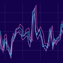
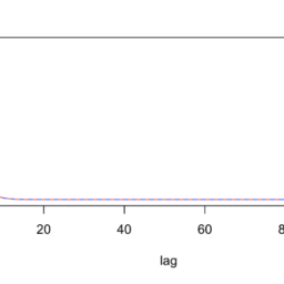
Question 1.2. The sample autocorrelation is perhaps the second most common type of plot in time series analysis, after simply plotting the data. We investigate how $R$ represents chance variation in the plot of the sample autocorrelation function produced by the acf function. We seek to check what R actually does when it constructs the dashed horizontal lines in this plot. What approximation is being made? How should the lines be interpreted statistically?
If you type acf in R, you get the source code for the acf function. You’ll see that the plotting is done by a service function plot. acf . This service function is part of the package, and is not immediately accessible to you. Nevertheless, you can check the source code as follows:
- Notice, either from the help documentation ?acf or the last line of the source code acf that this function resides in the package stats.
- Now, you can access this namespace directly, to list the source code, by
stats:: :plot. acf - Now we can see how the horizontal dashed lines are constructed. The critical line of code seems to be
$\operatorname{clim} 0<-$ if (with. ci) qnorm $((1+\operatorname{ci}) / 2) / \operatorname{sqrt}(x \$ n$. used)
This appears to correspond to a normal distribution approximation for the sample autocorrelation estimator, with mean zero and standard deviation $1 / \sqrt{N}$.
$$
\hat{\gamma}h\left(y{1: N}\right)=\frac{1}{N} \sum_{n=1}^{N-h}\left(y_n-\hat{\mu}n\right)\left(y{n+h}-\hat{\mu}{n+h}\right) . $$ Here, we consider the null hypothesis where $Y{1: N}$ is IID with mean 0 and standard deviation $\sigma$. We therefore use the estimator $\hat{\mu}n=0$ and the autocovariance function estimator becomes $$ \hat{\gamma}_h\left(y{1: N}\right)=\frac{1}{N} \sum_{n=1}^{N-h} y_n y_{n+h},
$$
We let $\sum_{n=1}^{N-h} Y_n Y_{n+h}=U$ and $\sum_{n=1}^N Y_n^2=V$, and carry out a first order Taylor expansion of
$$
\hat{\rho}h\left(Y{1: N}\right)=\frac{\hat{\gamma}h\left(y{1: N}\right)}{\hat{\gamma}0\left(y{1: N}\right)}=\frac{U}{V}
$$
about $(\mathbb{E}[U], \mathbb{E}[V])$. This gives
$$
\hat{\rho}h\left(Y{1: N}\right) \approx \frac{\mathbb{E}(U)}{\mathbb{E}(V)}+\left.(U-\mathbb{E}(U)) \frac{\partial}{\partial U}\left(\frac{U}{V}\right)\right|{(\mathbb{E}(U), \mathbb{E}(V))}+\left.(V-\mathbb{E}(V)) \frac{\partial}{\partial V}\left(\frac{U}{V}\right)\right|{(\mathbb{E}(U), \mathbb{E}(V))}
$$

MY-ASSIGNMENTEXPERT™可以为您提供UNIVERSITY OF ILLINOIS URBANA-CHAMPAIGN MATH2940 linear algebra线性代数课程的代写代考和辅导服务! 请认准MY-ASSIGNMENTEXPERT™. MY-ASSIGNMENTEXPERT™为您的留学生涯保驾护航。