MY-ASSIGNMENTEXPERT™可以为您提供 utstat.utoronto Stats531 Time series analysis时间序列分析的代写代考和辅导服务!
这是密歇根安娜堡的大学 时间序列分析的代写成功案例。
Stats531课程简介
Course description
This course gives an introduction to time series analysis using time domain methods and frequency domain methods. The goal is to acquire the theoretical and computational skills required to investigate data collected as a time series. The first half of the course will develop classical time series methodology, including auto-regressive moving average (ARMA) models, regression with ARMA errors, and estimation of the spectral density. The second half of the course will focus on state space model techniques for fitting structured dynamic models to time series data. We will progress from fitting linear, Gaussian dynamic models to fitting nonlinear models for which Monte Carlo methods are required. Examples will be drawn from ecology, economics, epidemiology, finance and elsewhere.
Prerequisites
Grading
Weekly homeworks (25%, due Tuesdays, in class).
A midterm exam (25%, in class on Thursday 2/25).
A midterm project analyzing a time series of your choice using methods covered in the first half of the course (15%, due Thursday 3/10).
A final project analyzing a time series of your choice using methods covered in the entire course (35%, due Thursday 4/28).
Discussion of homework problems is encouraged, but solutions must be written up individually. Direct copying is not acceptable.
Any material taken from any source, such as the internet, must be properly acknowledged. Unattributed copying from any source is plagiarism, and has potentially serious consequences.
Stats531 Time series analysis HELP(EXAM HELP, ONLINE TUTOR)
Question 2.1. We investigate two ways to calculate the autocovariance function for an ARMA model. The instructions below help you work through the case of a causal AR(1) model,
$$
X_n=\phi X_{n-1}+\epsilon_n
$$
where $\left{\epsilon_n\right}$ is white noise with variance $\sigma^2$, and $-1<\phi<1$. Assume the process is stationary, i.e., it is initialized with a random draw from its stationary distribution. Show your working for both the approaches $\mathrm{A}$ and $\mathrm{B}$ explained below. If you want an additional challenge, you can work through the $A R(2)$ or $\operatorname{ARMA}(1,1)$ case instead.
A. Using the stochastic difference equation to obtain a difference equation for the autocovariance function (ACF). Start by writing the ACF as
$$
\gamma_h=\operatorname{Cov}\left(X_n, X_{n+h}\right)=\operatorname{Cov}\left(X_n, \phi X_{n+h-1}+\epsilon_{n+h}\right), \text { for } h>0
$$
Writing the right hand side in terms of $\gamma_{h-1}$ leads to an equation which is formally a first order linear homogeneous recurrence relation with constant coefficients. To solve such an equation, we look for solutions of the form
$$
\gamma_h=A \lambda^h
$$
Substituting this general solution into the recurrence relation, together with an initial condition derived from explicitly computing $\gamma_0$, provides an approach to finding two equations that can be solved for the two unknowns, $A$ and $\lambda$.
B. Via the $\mathrm{MA}(\infty)$ representation. Construct a Taylor series expansion of $g(x)=(1-\phi x)^{-1}$ of the form
$$
g(x)=g_0+g_1 x+g_2 x^2+g_3 x^3+\ldots
$$
Do this either by hand or using your favorite math software (if you use software, please say what software you used and what you entered to get the output). Use this Taylor series to write down the $M A(\infty)$ representation of an AR(1) model. Then, apply the general formula for the autocovariance function of an $\mathrm{MA}(\infty)$ process.
C. Check your work for the specific case of an AR(1) model with $\phi_1=0.6$ by comparing your formula with the result of the $\mathrm{R}$ function ARMAacf .
Question 2.1.
A. Since $\left{\epsilon_n\right}$ is white noise with variance $\sigma^2$, then
$$
\begin{aligned}
\gamma_h & =\operatorname{Cov}\left(X_n, X_{n+h}\right) \
& =\operatorname{Cov}\left(X_n, \phi X_{n+h-1}+\epsilon_{n+h}\right) \
& =\phi \operatorname{Cov}\left(X_n, X_{n+h-1}\right)+\operatorname{Cov}\left(X_n, \epsilon_{n+h}\right) \
& =\phi \gamma_{h-1} .
\end{aligned}
$$
We can get $\gamma_0$ by simple computing,
$$
\begin{aligned}
\gamma_0 & =\operatorname{Cov}\left(X_n, X_n\right) \
\gamma_0 & =\operatorname{Cov}\left(\phi X_{n-1}+\epsilon_n, \phi X_{n-1}+\epsilon_n\right) \
\gamma_0 & =\phi^2 \operatorname{Cov}\left(X_{n-1}, X_{n-1}\right)+\operatorname{Cov}\left(\epsilon_n, \epsilon_n\right) \
\gamma_0 & =\phi^2 \gamma_0+\sigma^2 \
\left(1-\phi^2\right) \gamma_0 & =\sigma^2 \
\gamma_0 & =\frac{\sigma^2}{1-\phi^2}
\end{aligned}
$$
Let $\gamma_h=A \lambda^h$, then
$$
\begin{aligned}
A \lambda^h & =\phi \mathrm{R} \lambda^{h-1} \
\lambda^h & =\phi \lambda^{h-1} \
\lambda & =\phi .
\end{aligned}
$$
Applying $\gamma_0$ as an initial condition, then
$$
\begin{aligned}
A \lambda^0 & =\gamma_0 \
& =\frac{\sigma^2}{1-\phi^2}
\end{aligned}
$$
B. By Taylor series expansion,
$$
g(x)=g(0)+g^{\prime}(0) x+\frac{1}{2} g^{(2)}(0) x^2+\frac{1}{3 !} g^{(3)}(0) x^3+\ldots
$$
Since
$$
\begin{aligned}
g^{(n)}(0) & =\frac{d^n}{d t^n} \frac{1}{1-\phi x} \
& =n ! \phi^n x^n,
\end{aligned}
$$
we have
$$
g(x)=\sum_{n=0}^{\infty} \phi^n x^n
$$
The AR(1) model is equivalent to the following MA $(\infty)$ process
$$
\begin{aligned}
X_n & =\phi X_{n-1}+\epsilon_n \
& =\phi B X_n+\epsilon_n \
(1-\phi B) X_n & =\epsilon_n \
X_n & =(1-\phi B)^{-1} \epsilon_n \
& =\epsilon_n+\phi B \epsilon_n+\phi^2 B^2 \epsilon_n+\ldots \
& =\epsilon_n+\phi \epsilon_{n-1}+\phi^2 \epsilon_{n-2}+\ldots \
& =\sum_{j=0}^{\infty} \phi^j \epsilon_{n-j} .
\end{aligned}
$$
Then, apply the general formular for the autocovariance function of the MA $(\infty)$ process with the constraint $-1<\phi<1$,
$$
\begin{aligned}
\gamma_h & =\sum_{j=0}^{\infty} \psi_j \psi_{j+h} \sigma^2 \
& =\sum_{j=0}^{\infty} \phi^{2 j+h} \sigma^2 \
& =\phi^h \sigma^2 \sum_{j=0}^{\infty} \phi^{2 j} \
& =\frac{\phi^h \sigma^2}{1-\phi^2} .
\end{aligned}
$$
which is the same as the answer in $A$.
C. From the above derivation, we have
$$
\begin{aligned}
\rho_h & =\frac{\gamma_h}{\gamma_0} \
& =\frac{\frac{\phi^h \sigma^2}{1-\phi^2}}{\frac{\sigma^2}{1-\phi^2}} \
& =\phi^h
\end{aligned}
$$
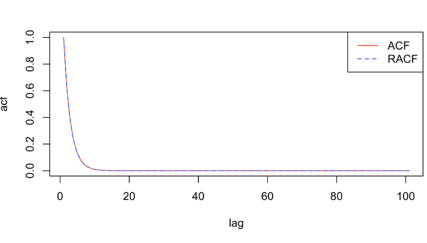
which is the same as R funtion ARMAacf by the following code.
HH [1] TRUE
plot (acf, type=” $1^{\prime \prime}$, col=’ red’, $\left.x l a b=”{ }^{\prime \prime} \mathrm{agg}^{\prime \prime}\right)$
lines (Racf, lty $=2$, col=’blue’)
legend (“topright”, legend $=\mathrm{c}($ “ACF”, “RaCF”), col =c(“red”, “blue”), lty $=\mathrm{c}(1,2))$
Question 2.2 Compute the autocovariance function (ACF) of the random walk model. Specifically, find the ACF, $\gamma_{m n}=\operatorname{Cov}\left(X_m, X_n\right)$, for the random walk model specified by
$$
X_n=X_{n-1}+\epsilon_n
$$
where $\left{\epsilon_n\right}$ is white noise with variance $\sigma^2$, and we use the initial value $X_0=0$.
Reading. We have covered much of the material through to Section 3.4 of Shumway and Stoffer (Time Series Analysis and its Applications, 3rd edition). The course notes are intended to be self-contained, and additional reading is therefore optional. Reading this textbook will help to broaden your understanding of these topics.
Question 2.2.
The solution of stochastic difference equation of the random walk model is:
$$
X_n=\sum_{k=1}^n \epsilon_k
$$
Therefore,
$$
\begin{aligned}
\gamma_{m n} & =\operatorname{Cov}\left(X_m, X_n\right) \
& =\operatorname{Cov}\left(\sum_{i=1}^n \epsilon_i, \sum_{j=1}^n \epsilon_j\right) \
& =\sum_{i=1}^{\min (m, n)} \operatorname{Var}\left(\epsilon_i\right) \
& =\min (m, n) \sigma^2
\end{aligned}
$$
Putting together, we have,
$$
\gamma_{m n}=\min (m, n) \sigma^2
$$

MY-ASSIGNMENTEXPERT™可以为您提供UNIVERSITY OF ILLINOIS URBANA-CHAMPAIGN MATH2940 linear algebra线性代数课程的代写代考和辅导服务! 请认准MY-ASSIGNMENTEXPERT™. MY-ASSIGNMENTEXPERT™为您的留学生涯保驾护航。