MY-ASSIGNMENTEXPERT™可以为您提供 utstat.utoronto Stats531 Time series analysis时间序列分析的代写代考和辅导服务!
这是密歇根安娜堡的大学 时间序列分析的代写成功案例。
Stats531课程简介
Course description
This course gives an introduction to time series analysis using time domain methods and frequency domain methods. The goal is to acquire the theoretical and computational skills required to investigate data collected as a time series. The first half of the course will develop classical time series methodology, including auto-regressive moving average (ARMA) models, regression with ARMA errors, and estimation of the spectral density. The second half of the course will focus on state space model techniques for fitting structured dynamic models to time series data. We will progress from fitting linear, Gaussian dynamic models to fitting nonlinear models for which Monte Carlo methods are required. Examples will be drawn from ecology, economics, epidemiology, finance and elsewhere.
Prerequisites
Grading
Weekly homeworks (25%, due Tuesdays, in class).
A midterm exam (25%, in class on Thursday 2/25).
A midterm project analyzing a time series of your choice using methods covered in the first half of the course (15%, due Thursday 3/10).
A final project analyzing a time series of your choice using methods covered in the entire course (35%, due Thursday 4/28).
Discussion of homework problems is encouraged, but solutions must be written up individually. Direct copying is not acceptable.
Any material taken from any source, such as the internet, must be properly acknowledged. Unattributed copying from any source is plagiarism, and has potentially serious consequences.
Stats531 Time series analysis HELP(EXAM HELP, ONLINE TUTOR)
(1) Estimate the trend of the series of gasoline consumption in Spain using a straight line in the period from 1945 to 1995 and generate forecasts for 24 months. Compare the results with Holt’s method.
(2) Apply a decomposition method to the gasoline consumption series and estimate the seasonal coefficients. Compare the results when Holt’s method and using moving averages.
(3) Obtain the periodogram for the series of Columbus’s voyage and interpret it.
(4) Obtain the periodogram for the gasoline consumption series and interpret it.
(5) Prove that the predictions made using Holt’s method verify the recursive equation- $\widehat{z}{T+1}(1)=\widehat{z}_T(1)+$ $\widehat{\beta}_T+\gamma(1-\theta)\left(z{T+1-} \widehat{\mu}_T-\widehat{\beta}_T\right)$
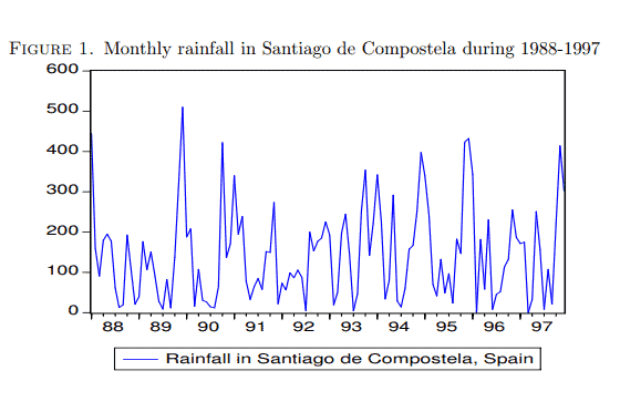
(1) Figure 1 shows monthly rainfall in Santiago de Compostela during the years 1988-1997. Would it be a stationary process?
(2) Let us consider the process $z_t=.5 z_{t-1}+a_t$ where $a_t$ is a white noise process. Calculate the marginal mean, its variance and first order autocovariance. Is the process stationary?
(3) In the above exercise, calculate the expectation and variance of the conditional distribution $f\left(z_t \mid z_{t-1}\right)$. Compare these results with those obtained in the above exercise for the marginal distribution.
(4) Let us consider the process $z_t=-.5 a_{t-1}+a_t$. Calculate its mean and first and second order autocovariance. Is the process stationary?
(5) Prove that the above process can be written as $z_t=-.5\left(z_{t-1}+.5 a_{t-2}\right)+a_t=-.5 z_{t-1}-.25 a_{t-2}+a_t$. Use this equation to calculate the expectation and variance of the conditional distribution $f\left(z_t \mid z_{t-1}\right)$. Compare the results with those of the marginal distribution.
(6) Given a stationary series, prove that if the autocovariances are all positive then the mean of the process will be estimated with greater variance than if all the autocovariances are null.
(7) Prove that the mean of the process in exercise (4) is estimated with less variability than in a process with independent data and the same marginal variance.
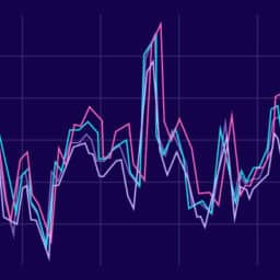
(1) Generate samples of an AR(1) process with $\phi=.7$ using a computer program as follows: (1) generate a vector $a_t$ of 150 random normal variables $(0,1) ;(2)$ take $z_1=a_1 ;(3)$ for $t=2, \ldots, 150$ calculate $z_t=$ $.7 z_{t-1}+a_t ;$ (4) to avoid the effect of the initial conditions, eliminate the first 50 observations and take the values $z_{51}, \ldots z_{150}$ as a sample of 100 of the AR(1) process.
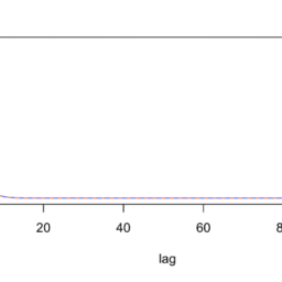
(2) Obtain the theoretical autocorrelation function of the process $z_t=.7 z_{t-1}+a_t$, where $a_t$ is white noise. Compare the theoretical results with those observed in the sample from the above exercise.
(3) Obtain the theoretical autocorrelation function of the process $z_t=.9 z_{t-1}-.18 z_{t-1}+a_t$, where $a_t$ is white noise. Generate a realization of the process using a computer and compare the sample function with the theoretical one.
(4) Express in operator notation the processes of exercises (2) and (3). Represent the process in the form $z_t=\sum \psi_i a_{t-i}$ obtaining the inverse operators.
(5) Write the theoretical autocorrelation function of the process $\left(1-1.2 B+.32 B^2\right) z_t=a_t$. Obtain the representation of this process as $z_t=\sum \psi_i a_{t-i}$ and comment on the relationship between the coefficients $\psi$ and the autocorrelation function.

MY-ASSIGNMENTEXPERT™可以为您提供 UTSTAT.UTORONTO STATS531 TIME SERIES ANALYSIS时间序列分析的代写代考和辅导服务!