如果你也在 怎样代写机器学习Machine Learning 这个学科遇到相关的难题,请随时右上角联系我们的24/7代写客服。机器学习Machine Learning是一个致力于理解和建立 “学习 “方法的研究领域,也就是说,利用数据来提高某些任务的性能的方法。机器学习算法基于样本数据(称为训练数据)建立模型,以便在没有明确编程的情况下做出预测或决定。机器学习算法被广泛用于各种应用,如医学、电子邮件过滤、语音识别和计算机视觉,在这些应用中,开发传统算法来执行所需任务是困难的或不可行的。
机器学习Machine Learning程序可以在没有明确编程的情况下执行任务。它涉及到计算机从提供的数据中学习,从而执行某些任务。对于分配给计算机的简单任务,有可能通过编程算法告诉机器如何执行解决手头问题所需的所有步骤;就计算机而言,不需要学习。对于更高级的任务,由人类手动创建所需的算法可能是一个挑战。在实践中,帮助机器开发自己的算法,而不是让人类程序员指定每一个需要的步骤,可能会变得更加有效 。
机器学习Machine Learning代写,免费提交作业要求, 满意后付款,成绩80\%以下全额退款,安全省心无顾虑。专业硕 博写手团队,所有订单可靠准时,保证 100% 原创。 最高质量的机器学习Machine Learning作业代写,服务覆盖北美、欧洲、澳洲等 国家。 在代写价格方面,考虑到同学们的经济条件,在保障代写质量的前提下,我们为客户提供最合理的价格。 由于作业种类很多,同时其中的大部分作业在字数上都没有具体要求,因此机器学习Machine Learning作业代写的价格不固定。通常在专家查看完作业要求之后会给出报价。作业难度和截止日期对价格也有很大的影响。
同学们在留学期间,都对各式各样的作业考试很是头疼,如果你无从下手,不如考虑my-assignmentexpert™!
my-assignmentexpert™提供最专业的一站式服务:Essay代写,Dissertation代写,Assignment代写,Paper代写,Proposal代写,Proposal代写,Literature Review代写,Online Course,Exam代考等等。my-assignmentexpert™专注为留学生提供Essay代写服务,拥有各个专业的博硕教师团队帮您代写,免费修改及辅导,保证成果完成的效率和质量。同时有多家检测平台帐号,包括Turnitin高级账户,检测论文不会留痕,写好后检测修改,放心可靠,经得起任何考验!
想知道您作业确定的价格吗? 免费下单以相关学科的专家能了解具体的要求之后在1-3个小时就提出价格。专家的 报价比上列的价格能便宜好几倍。
我们在计算机Quantum computer代写方面已经树立了自己的口碑, 保证靠谱, 高质且原创的计算机Quantum computer代写服务。我们的专家在机器学习Machine Learning代写方面经验极为丰富,各种机器学习Machine Learning相关的作业也就用不着 说。
计算机代写|机器学习代写Machine Learning代考|Learning undirected graph structures
In this section, we discuss how to learn the structure of undirected graphical models. On the one hand, this is easier than learning DAG structure because we don’t need to worry about acyclicity. On the other hand, it is harder than learning DAG structure since the likelihood does not decompose (see ??). This precludes the kind of local search methods both greedy search and MCMC sampling we used to learn DAG structures, because the cost of evaluating each neighboring graph is too high, since we have to refit each model from scratch (there is no way to incrementally update the score of a model). In this section, we discuss several solutions to this problem.
A simple way to learn the structure of a UGM is to represent it is as a product of full conditionals:
$$
p(\boldsymbol{x})=\frac{1}{Z} \prod_{d=1}^D p\left(x_d \mid \boldsymbol{x}_{-d}\right)
$$
This expression is called the pseudolikelihood.
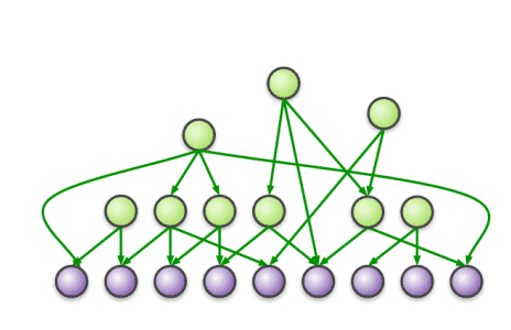
Such a collection of local distributions defines a model called a dependency network [Hec +00$]$. Unfortunately, a product of full conditionals which are independently estimated is not guaranteed to be consistent with any valid joint distribution. However, we can still use the model inside of a Gibbs sampler to approximate a joint distribution. This approach is sometimes used for data imputation GR01.
However, the main use advantage of dependency networks is that we can use sparse regression techniques for each distribution $p\left(x_d \mid \boldsymbol{x}_{-d}\right)$ to induce a sparse graph structure. For example, [Hec+00] use classification/ regression trees, MB06 use $\ell_1$-regularized linear regression, WRL06; WSD19 use $\ell_1$-regularized logistic regression, Dob09 uses Bayesian variable selection, etc.
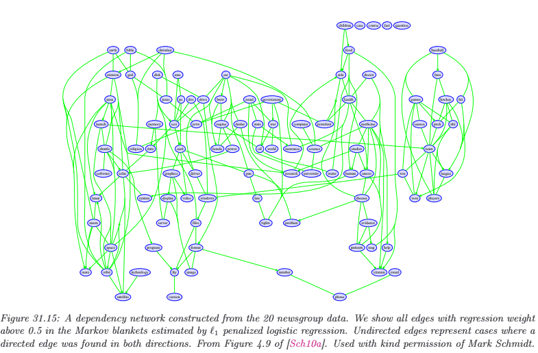
Figure 31.15 shows a dependency network that was learned from the 20 -newsgroup data using $\ell_1$ regularized logistic regression, where the penalty parameter $\lambda$ was chosen by BIC. Many of the words present in these estimated Markov blankets represent fairly natural associations aids:disease, baseball:fans, bible:god, bmw:car, cancer:patients, etc. However, some of the estimated statistical dependencies seem less intuitive, such as baseball:windows and bmw:christian. We can gain more insight if we look not only at the sparsity pattern, but also the values of the regression weights. For example, here are the incoming weights for the first 5 words:
- aids: children $(0.53)$, disease $(0.84)$, fact $(0.47)$, health $(0.77)$, president $(0.50)$, research $(0.53)$
- baseball: christian $(-0.98)$, drive $(-0.49)$, games $(0.81)$, god $(-0.46)$, government $(-0.69)$, hit $(0.62)$, memory $(-1.29)$, players $(1.16)$, season $(0.31)$, software $(-0.68)$, windows $(-1.45)$
- bible: car $(-0.72)$, card $(-0.88)$, christian $(0.49)$, fact $(0.21)$, god (1.01), jesus $(0.68)$, orbit $(0.83)$, program $(-0.56)$, religion $(0.24)$, version $(0.49)$
- bmw: car (0.60), christian (-11.54), engine $(0.69), \operatorname{god}(-0.74)$, government $(-1.01)$, help $(-0.50)$, windows $(-1.43)$
- cancer: disease $(0.62)$, medicine $(0.58)$, patients $(0.90)$, research $(0.49)$, studies $(0.70)$
Words in italic red have negative weights, which represents a dissociative relationship. For example, the model reflects that baseball:windows is an unlikely combination. It turns out that most of the weights are negative ( 1173 negative, 286 positive, 8541 zero) in this model.
计算机代写|机器学习代写Machine Learning代考|Graphical lasso for GGMs
Before discussing structure learning, we need to discuss parameter estimation. The task of computing the MLE for a (non-decomposable) GGM is called covariance selection [Dem72].
The log likelihood can be written as
$$
\ell(\boldsymbol{\Omega})=\log \operatorname{det} \boldsymbol{\Omega}-\operatorname{tr}(\mathbf{S} \boldsymbol{\Omega})
$$
where $\boldsymbol{\Omega}=\boldsymbol{\Sigma}^{-1}$ is the precision matrix, and $\mathbf{S}=\frac{1}{N} \sum_{i=1}^N\left(\boldsymbol{x}i-\overline{\boldsymbol{x}}\right)\left(\boldsymbol{x}_i-\overline{\boldsymbol{x}}\right)^{\boldsymbol{\top}}$ is the empirical covariance matrix. (For notational simplicity, we assume we have already estimated $\hat{\boldsymbol{\mu}}=\overline{\boldsymbol{x}}$.) One can show that the gradient of this is given by $$ \nabla \ell(\Omega)=\Omega^{-1}-\mathbf{S} $$ However, we have to enforce the constraints that $\Omega{s t}=0$ if $G_{s t}=0$ (structural zeros), and that $\boldsymbol{\Omega}$ is positive definite. The former constraint is easy to enforce, but the latter is somewhat challenging (albeit still a convex constraint). One approach is to add a penalty term to the objective if $\boldsymbol{\Omega}$ leaves the positive definite cone; this is the approach used in [DVR08]. Another approach is to use a coordinate descent method, described in $[\mathrm{HTF} 09, \mathrm{p} 633]$
Interestingly, one can show that the MLE must satisfy the following property: $\Sigma_{s t}=S_{s t}$ if $G_{s t}=1$ or $s=t$, i.e., the covariance of a pair that are connected by an edge must match the empirical covariance. In addition, we have $\Omega_{s t}=0$ if $G_{s t}=0$, by definition of a GGM, i.e., the precision of a pair that are not connected must be 0 . We say that $\mathbf{\Sigma}$ is a positive definite matrix completion of $\mathbf{S}$, since it retains as many of the entries in $\mathbf{S}$ as possible, corresponding to the edges in the graph, subject to the required sparsity pattern on $\boldsymbol{\Sigma}^{-1}$, corresponding to the absent edges; the remaining entries in $\boldsymbol{\Sigma}$ are filled in so as to maximize the likelihood.
机器学习代写
计算机代写|机器学习代写MACHINE LEARNING代考|LEARNING UNDIRECTED GRAPH STRUCTURES
在本节中,我们将讨论如何学习无向图模型的结构。一方面,这比学习 DAG 结构更容易,因为我们不需要担心无环性。另一方面,它比学习 DAG 结构更难,因为可能性不会分解see??. 这排除了我们用于学习 DAG 结构的贪婪搜索和 MCMC 采样的那种局部搜索方法,因为评估每个相邻图的成 本太高,因为我们必须从头开始重新拟合每个模型thereisnowaytoincrementallyupdatethescoreofamodel. 在本节中,我们将讨论此问题的 几种解决方案。
学习 UGM 结构的一种简单方法是将其表示为完整条件的乘积:
$$
p(\boldsymbol{x})=\frac{1}{Z} \prod_{d=1}^D p\left(x_d \mid \boldsymbol{x}{-d}\right) $$ 该表达式称为伪似然。 这样的局部分布集合定义了一个称为依赖网络的模型 $$ \mathrm{Hec}+00 \$ $$ \$。不幸的是,独立估计的完整条件的乘积不能保证与任何有效的联合分布一致。但是,我们仍然可以使用 Gibbs 采样器内部的模型来近似联合分 布。这种方法有时用于数据揷补 GR01。 然而,依赖网络的主要使用优势是我们可以对每个分布使用稀疏回归技术 $p\left(x_d \mid \boldsymbol{x}{-d}\right)$ 诱导稀疏图结构。例如,
$$
H e c+00
$$
使用分类/回归树,MB06 使用 $\ell_1$-正则化线性回归,WRL06;WSD19使用 $\ell_1$-正则化逻辑回归,Dob09使用贝叶斯变量选择等
图 31.15 显示了从 20 -newsgroup 数据中学习的依赖网络 $\ell_1$ 正则化逻辑回归,其中惩罚参数 $\lambda$ 被 BIC 选择。这些估计的马尔可夫琰中出现的许多词代 表相当自然的关联 aids:disease、baseball:fans、bible:god、bmw:car、cancer:patients等。但是,一些估计的统计相关性似乎不太直观,例如棒 球:窗户和宝马:基督教。如果我们不仅查看稀疏模式,还查看回归权重的值,我们可以获得更多洞察力。例如,这里是前 5 个词的传入权重:
- 辅助工具: 儿童 $(0.53)$ ,疾病 $(0.84)$ ,事实 $(0.47)$ ,健康 $(0.77)$ ,总统 $(0.50)$ ,研究 $(0.53)$
- 棒球: 基督教 $(-0.98)$ ,驾驶 $(-0.49)$, 游戏 $(0.81)$ ,上帝 $(-0.46)$ ,政府 $(-0.69)$ ,打 $(0.62)$ ,记忆 $(-1.29)$, 球员 $(1.16)$ ,季节 $(0.31)$ , 软件 $(-0.68)$, 窗户 $(-1.45)$
- 圣经: 汽车 $(-0.72)$, 卡片 $(-0.88)$, 基督徒 $(0.49)$, 事实 $(0.21)$ ,上帝 1.01 , 耶稣 $(0.68)$, 轨道 $(0.83)$ ,程序 $(-0.56)$ ,宗教 $(0.24)$ ,版本 $(0.49)$
- 宝马: 汽车 0.60 ,基督徒 -11.54 ,引擎 $(0.69), \operatorname{god}(-0.74)$ ,政府 $(-1.01)$ ,帮助 $(-0.50)$,窗户 $(-1.43)$
- 㾔症: 疾病 $(0.62)$ ,药品 $(0.58)$ ,患者 $(0.90)$ ,研究(0.49),学习(0.70) 斜体红色的词具有负权重,代表分离关系。例如,该模型反映出 baseball:windows 是一个不太可能的组合。事实证明大部分权重都是负数 1173negative, 286positive, 8541zero在这个模型中。
计算机代写|机器学习代写MACHINE LEARNING代考|GRAPHICAL LASSO FOR GGMS
在讨论结构学习之前,我们需要讨论参数估计。计算 MLE 的任务non – decomposableGGM称为协方差选择
$\operatorname{Dem} 72$
对数似然可以写成
$$
\ell(\boldsymbol{\Omega})=\log \operatorname{det} \boldsymbol{\Omega}-\operatorname{tr}(\mathbf{S} \boldsymbol{\Omega})
$$
在哪里 $\boldsymbol{\Omega}=\boldsymbol{\Sigma}^{-1}$ 是精度矩阵,并且 $\mathbf{S}=\frac{1}{N} \sum_{i=1}^N(\boldsymbol{x} i-\overline{\boldsymbol{x}})\left(\boldsymbol{x}i-\overline{\boldsymbol{x}}\right)^{\top}$ 是经验协方差矩阵。 Fornotationalsimplicity, weassumewehavealreadyestimated $\$ \hat{\boldsymbol{\mu}}=\overline{\boldsymbol{x}} \$$. 可以证明其梯度由下式给出 $$ \nabla \ell(\Omega)=\Omega^{-1}-\mathbf{S} $$ 但是,我们必须强制执行以下约束 $\Omega s t=0$ 如果 $G{s t}=0$ structuralzeros,然后 $\Omega$ 是正定的。前者约束容易执行,但后者有点挑战性 albeitstillaconvexconstraint. 一种方法是在目标中添加一个従罚项,如果 $\Omega$ 离开正定雉;这是使用的方法
$D V R 08$
.另一种方法是使用坐标下降法,在[HTF09, p633]
有趣的是,可以证明 MLE 必须满足以下属性: $\Sigma_{s t}=S_{s t}$ 如果 $G_{s t}=1$ 或者 $s=t$ ,即由边连接的一对的协方差必须与经验协方差匹配。此外,我 们有 $\Omega_{s t}=0$ 如果 $G_{s t}=0$ ,根据 GGM 的定义,即末连接的一对的精度必须为 0 。我们说 $\mathbf{\Sigma}$ 是一个正定矩阵完成 $\mathbf{S}$ ,因为它保留了尽可能多的条目 $\mathbf{S}$ 尽可能对应于图中的边,受限于所需的稀疏模式 $\boldsymbol{\Sigma}^{-1}$, 对应于缺失的边;中的剩余条目 $\boldsymbol{\Sigma}$ 被填充以最大化可能性

计算机代写|机器学习代写Machine Learning代考 请认准UprivateTA™. UprivateTA™为您的留学生涯保驾护航。
微观经济学代写
微观经济学是主流经济学的一个分支,研究个人和企业在做出有关稀缺资源分配的决策时的行为以及这些个人和企业之间的相互作用。my-assignmentexpert™ 为您的留学生涯保驾护航 在数学Mathematics作业代写方面已经树立了自己的口碑, 保证靠谱, 高质且原创的数学Mathematics代写服务。我们的专家在图论代写Graph Theory代写方面经验极为丰富,各种图论代写Graph Theory相关的作业也就用不着 说。
线性代数代写
线性代数是数学的一个分支,涉及线性方程,如:线性图,如:以及它们在向量空间和通过矩阵的表示。线性代数是几乎所有数学领域的核心。
博弈论代写
现代博弈论始于约翰-冯-诺伊曼(John von Neumann)提出的两人零和博弈中的混合策略均衡的观点及其证明。冯-诺依曼的原始证明使用了关于连续映射到紧凑凸集的布劳威尔定点定理,这成为博弈论和数学经济学的标准方法。在他的论文之后,1944年,他与奥斯卡-莫根斯特恩(Oskar Morgenstern)共同撰写了《游戏和经济行为理论》一书,该书考虑了几个参与者的合作游戏。这本书的第二版提供了预期效用的公理理论,使数理统计学家和经济学家能够处理不确定性下的决策。
微积分代写
微积分,最初被称为无穷小微积分或 “无穷小的微积分”,是对连续变化的数学研究,就像几何学是对形状的研究,而代数是对算术运算的概括研究一样。
它有两个主要分支,微分和积分;微分涉及瞬时变化率和曲线的斜率,而积分涉及数量的累积,以及曲线下或曲线之间的面积。这两个分支通过微积分的基本定理相互联系,它们利用了无限序列和无限级数收敛到一个明确定义的极限的基本概念 。
计量经济学代写
什么是计量经济学?
计量经济学是统计学和数学模型的定量应用,使用数据来发展理论或测试经济学中的现有假设,并根据历史数据预测未来趋势。它对现实世界的数据进行统计试验,然后将结果与被测试的理论进行比较和对比。
根据你是对测试现有理论感兴趣,还是对利用现有数据在这些观察的基础上提出新的假设感兴趣,计量经济学可以细分为两大类:理论和应用。那些经常从事这种实践的人通常被称为计量经济学家。
Matlab代写
MATLAB 是一种用于技术计算的高性能语言。它将计算、可视化和编程集成在一个易于使用的环境中,其中问题和解决方案以熟悉的数学符号表示。典型用途包括:数学和计算算法开发建模、仿真和原型制作数据分析、探索和可视化科学和工程图形应用程序开发,包括图形用户界面构建MATLAB 是一个交互式系统,其基本数据元素是一个不需要维度的数组。这使您可以解决许多技术计算问题,尤其是那些具有矩阵和向量公式的问题,而只需用 C 或 Fortran 等标量非交互式语言编写程序所需的时间的一小部分。MATLAB 名称代表矩阵实验室。MATLAB 最初的编写目的是提供对由 LINPACK 和 EISPACK 项目开发的矩阵软件的轻松访问,这两个项目共同代表了矩阵计算软件的最新技术。MATLAB 经过多年的发展,得到了许多用户的投入。在大学环境中,它是数学、工程和科学入门和高级课程的标准教学工具。在工业领域,MATLAB 是高效研究、开发和分析的首选工具。MATLAB 具有一系列称为工具箱的特定于应用程序的解决方案。对于大多数 MATLAB 用户来说非常重要,工具箱允许您学习和应用专业技术。工具箱是 MATLAB 函数(M 文件)的综合集合,可扩展 MATLAB 环境以解决特定类别的问题。可用工具箱的领域包括信号处理、控制系统、神经网络、模糊逻辑、小波、仿真等。