如果你也在 怎样代写优化理论Optimization Theory 这个学科遇到相关的难题,请随时右上角联系我们的24/7代写客服。优化理论Optimization Theory是致力于解决优化问题的数学分支。 优化问题是我们想要最小化或最大化函数值的数学函数。 这些类型的问题在计算机科学和应用数学中大量存在。
优化理论Optimization Theory每个优化问题都包含三个组成部分:目标函数、决策变量和约束。 当人们谈论制定优化问题时,它意味着将“现实世界”问题转化为包含这三个组成部分的数学方程和变量。目标函数,通常表示为 f 或 z,反映要最大化或最小化的单个量。交通领域的例子包括“最小化拥堵”、“最大化安全”、“最大化可达性”、“最小化成本”、“最大化路面质量”、“最小化排放”、“最大化收入”等等。
优化理论Optimization Theory代写,免费提交作业要求, 满意后付款,成绩80\%以下全额退款,安全省心无顾虑。专业硕 博写手团队,所有订单可靠准时,保证 100% 原创。最高质量的优化理论Optimization Theory作业代写,服务覆盖北美、欧洲、澳洲等 国家。 在代写价格方面,考虑到同学们的经济条件,在保障代写质量的前提下,我们为客户提供最合理的价格。 由于作业种类很多,同时其中的大部分作业在字数上都没有具体要求,因此优化理论Optimization Theory作业代写的价格不固定。通常在专家查看完作业要求之后会给出报价。作业难度和截止日期对价格也有很大的影响。
同学们在留学期间,都对各式各样的作业考试很是头疼,如果你无从下手,不如考虑my-assignmentexpert™!
my-assignmentexpert™提供最专业的一站式服务:Essay代写,Dissertation代写,Assignment代写,Paper代写,Proposal代写,Proposal代写,Literature Review代写,Online Course,Exam代考等等。my-assignmentexpert™专注为留学生提供Essay代写服务,拥有各个专业的博硕教师团队帮您代写,免费修改及辅导,保证成果完成的效率和质量。同时有多家检测平台帐号,包括Turnitin高级账户,检测论文不会留痕,写好后检测修改,放心可靠,经得起任何考验!
想知道您作业确定的价格吗? 免费下单以相关学科的专家能了解具体的要求之后在1-3个小时就提出价格。专家的 报价比上列的价格能便宜好几倍。
我们在数学Mathematics代写方面已经树立了自己的口碑, 保证靠谱, 高质且原创的数学Mathematics代写服务。我们的专家在优化理论Optimization Theory代写方面经验极为丰富,各种优化理论Optimization Theory相关的作业也就用不着说。
数学代写|优化理论代写Optimization Theory代考|PONTRYAGIN’S MINIMUM PRINCIPLE AND STATE INEQUALITY CONSTRAINTS
So far, we have assumed that the admissible controls and states are not constrained by any boundaries; however, in realistic systems such constraints do commonly occur. Physically realizable controls generally have magnitude limitations: the thrust of a rocket engine cannot exceed a certain value; motors, which provide torque, saturate; attitude control mass expulsion systems are capable of providing a limited torque. State constraints often arise because of safety, or structural restrictions: the current in an electric motor cannot exceed a certain value without damaging the windings; the turning radius of a maneuvering aircraft cannot be less than a specified minimum value; a spacecraft reentering the earth’s atmosphere must satisfy certain attitude and velocity constraints to avoid burning up.
Let us first consider the effect of control constraints on the fundamental theorem derived in Section 4.1, and then show how the nećessary conditions are modified. $\dagger$ This generalization of the fundamental theorem leads to Pontryagin’s minimum principle.
Pontryagin’s Minimum Principle
By definition, the control $\mathbf{u}^$ causes the functional $J$ to have a relative minimum if $$ J(\mathbf{u})-J\left(\mathbf{u}^\right)=\Delta J \geq 0
$$
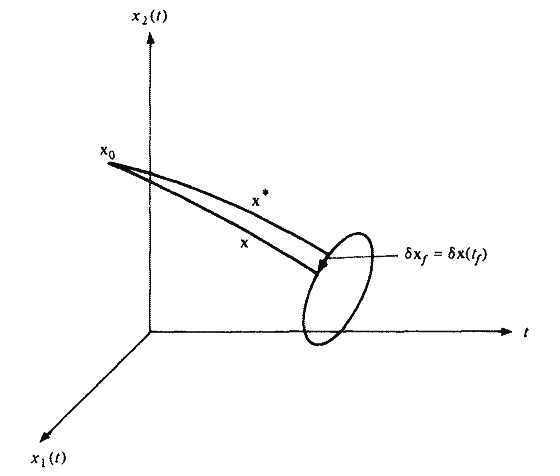
for all admissible controls sufficiently close to $\mathbf{u}^$. If we let $\mathbf{u}=\mathbf{u}^+\delta \mathbf{u}$, the increment in $J$ can be expressed as
$$
\Delta J\left(\mathbf{u}^, \delta \mathbf{u}\right)=\delta J\left(\mathbf{u}^, \delta \mathbf{u}\right)+\text { higher-order terms }
$$
$\delta J$ is linear in $\delta \mathbf{u}$ and the higher-order terms approach zero as the norm of $\delta$ approaches zero. If we were to re-prove the fundamental theorem for unbounded controls using control system notation, the reasoning would be exactly as given in Section 4.1. That is, if the control were unbounded, we could use the linearity of $\delta J$ with respect to $\delta \mathbf{u}$, and the fact that $\delta \mathbf{u}$ can vary arbitrarily to show that a necessary condition for $\mathbf{u}^$ to be an extremal control is that the variation $\delta J\left(\mathbf{u}^, \delta \mathbf{u}\right)$ must be zero for all admissible $\delta \mathbf{u}$ having a sufficiently small norm. Since we are no longer assuming that the admissible controls are not bounded, $\delta \mathbf{u}$ is arbitrary only if the extremal control is strictly within the boundary for all time in the interval $\left[t_0, t_f\right]$. In this case, the boundary has no effect on the problem solution. If, however, an extremal control lies on a boundary during at least one subinterval $\left[t_1, t_2\right]$ of the interval $\left[t_0, t_f\right]$, as shown in Fig. 5-13(a), then admissible control variations $\delta \hat{\mathbf{u}}$ exist whose negatives $(-\delta \hat{u})$ are not admissible. One such control variation is shown in Fig. 5-13(b). If only these variations are considered, a necessary condition for $\mathbf{u}^$ to minimize $J$ is that $\delta J\left(\mathbf{u}^, \delta \hat{\mathbf{u}}\right) \geq 0$. On the other hand, for variations
$\delta \tilde{u}$, which are nonzero only for $t$ not in the interval $\left[t_1, t_2\right]$, as, for example, in Fig. $5-13(\mathrm{c})$, it is necessary that $\delta J\left(\mathbf{u}^, \delta \tilde{u}\right)=0$; the reasoning used in proving the fundamental theorem applies. Considering all admissible variations with $|\delta \mathbf{u}|$ small enough so that the sign of $\Delta J$ is determined by $\delta J$, we see that a necessary condition for $\mathbf{u}^$ to minimize $J$ is
$$
\delta J\left(\mathbf{u}^*, \delta \mathbf{u}\right) \geq 0
$$
数学代写|优化理论代写Optimization Theory代考|Additional Necessary Conditions
Pontryagin and his co-workers have also derived other necessary conditions for optimality that we will find useful. We now state, without proof, two of these necessary conditions:
If the final time is fixed and the Hamiltonian does not depend explicitly on time, then the Hamiltonian must be a constant when evaluated on an extremal trajectory; that is,
$$
\mathscr{H}\left(\mathbf{x}^(t), \mathbf{u}^(t), \mathbf{p}^*(t)\right)=c_1 \quad \text { for } t \in\left[t_0, t_f\right]
$$
If the final time is free, and the Hamiltonian does not explicitly depend on time, then the Hamiltonian must be identically zero when evaluated on an extremal trajectory; that is,
$$
\mathscr{H}\left(\mathbf{x}^(t), \mathbf{u}^(t), \mathbf{p}^*(t)\right)=0 \quad \text { for } t \in\left[t_0, t_f\right]
$$
State Variable Inequality Constraints
Let us now consider problems in which there may be inequality constraints that involve the state variables as well as the controls. It will be assumed that the state constraints are of the form
$$
\mathbf{f}(\mathbf{x}(t), t) \geq \mathbf{0 , \dagger}
$$
where $\mathbf{f}$ is an $l$-vector function $(l \leq m)$ of the states and possibly time, which has continuous first and second partial derivatives with respect to $\mathbf{x}(t)$. It will also be assumed that the admissible control values lie in a closed and bounded region. Our approach will be to transform the $l$ inequality constraints of (5.3-42) into a single equality constraint, and then to augment the performance measure with this equality constraint, as we have done previously with the state equations.
优化理论代写
数学代写|优化理论代写Optimization Theory代考|PONTRYAGIN’S MINIMUM PRINCIPLE AND STATE INEQUALITY CONSTRAINTS
到目前为止,我们假设允许的控制和状态不受任何边界的约束;然而,在现实系统中,这样的约束确实经常发生。物理上可实现的控制通常有大小限制:火箭发动机的推力不能超过一定值;电机,提供扭矩,饱和;姿态控制排气系统能够提供有限的扭矩。由于安全或结构的限制,通常会出现状态约束:电动机中的电流不能超过一定值而不损坏绕组;机动飞行器的转弯半径不能小于规定的最小值;航天器重返地球大气层必须满足一定的姿态和速度限制,以避免燃烧。
让我们首先考虑控制约束对4.1节中导出的基本定理的影响,然后展示如何修改nećessary条件。$\dagger$这个基本定理的推广引出了庞特里亚金最小原理。
Pontryagin最小原则
根据定义,如果$$ J(\mathbf{u})-J\left(\mathbf{u}^\right)=\Delta J \geq 0
$$
对于所有允许的控件足够接近$\mathbf{u}^$,则控制$\mathbf{u}^$使函数$J$具有相对最小值。如果我们令$\mathbf{u}=\mathbf{u}^+\delta \mathbf{u}$,则$J$中的增量可以表示为
$$
\Delta J\left(\mathbf{u}^, \delta \mathbf{u}\right)=\delta J\left(\mathbf{u}^, \delta \mathbf{u}\right)+\text { higher-order terms }
$$
$\delta J$在$\delta \mathbf{u}$中是线性的,并且随着$\delta$的范数趋于零,高阶项趋于零。如果我们要用控制系统符号重新证明无界控制的基本定理,其推理将完全如第4.1节所述。也就是说,如果控制是无界的,我们可以使用$\delta J$相对于$\delta \mathbf{u}$的线性,并且$\delta \mathbf{u}$可以任意变化的事实表明,$\mathbf{u}^$成为极端控制的必要条件是,对于所有允许的$\delta \mathbf{u}$具有足够小的范数,变化$\delta J\left(\mathbf{u}^, \delta \mathbf{u}\right)$必须为零。因为我们不再假设允许的控制是无界的,所以$\delta \mathbf{u}$是任意的,只有当极限控制严格地在区间$\left[t_0, t_f\right]$的所有时间内的边界内。在这种情况下,边界对问题的解决没有影响。然而,如果在区间$\left[t_0, t_f\right]$的至少一个子区间$\left[t_1, t_2\right]$的边界上有一个极值控制,如图5-13(a)所示,则存在可容许的控制变异$\delta \hat{\mathbf{u}}$,其负$(-\delta \hat{u})$是不可容许的。图5-13(b)显示了一种这样的控制变化。如果只考虑这些变化,那么$\mathbf{u}^$使$J$最小化的一个必要条件是$\delta J\left(\mathbf{u}^, \delta \hat{\mathbf{u}}\right) \geq 0$。另一方面,对于变化
$\delta \tilde{u}$,它只在$t$不在$\left[t_1, t_2\right]$区间内是非零的,例如图$5-13(\mathrm{c})$,则需要$\delta J\left(\mathbf{u}^, \delta \tilde{u}\right)=0$;用来证明基本定理的推理是适用的。考虑到$|\delta \mathbf{u}|$的所有允许的变化都足够小,以至于$\Delta J$的符号由$\delta J$决定,我们看到$\mathbf{u}^$使$J$最小的必要条件是
$$
\delta J\left(\mathbf{u}^*, \delta \mathbf{u}\right) \geq 0
$$
数学代写|优化理论代写Optimization Theory代考|Additional Necessary Conditions
庞特里亚金和他的同事们还推导出了我们认为有用的其他最优性的必要条件。我们现在在没有证据的情况下陈述其中两个必要条件:
如果最终时间是固定的,并且哈密顿量不显式地依赖于时间,那么在极值轨迹上计算哈密顿量时必须是常数;也就是说,
$$
\mathscr{H}\left(\mathbf{x}^(t), \mathbf{u}^(t), \mathbf{p}^(t)\right)=c_1 \quad \text { for } t \in\left[t_0, t_f\right] $$ 如果最终时间是自由的,并且哈密顿量不显式地依赖于时间,那么在极值轨迹上计算哈密顿量时,哈密顿量必须等于零;也就是说, $$ \mathscr{H}\left(\mathbf{x}^(t), \mathbf{u}^(t), \mathbf{p}^(t)\right)=0 \quad \text { for } t \in\left[t_0, t_f\right]
$$
状态变量不等式约束
现在让我们考虑一些问题,其中可能存在不平等约束,包括状态变量和控制。假定状态约束的形式为
$$
\mathbf{f}(\mathbf{x}(t), t) \geq \mathbf{0 , \dagger}
$$
其中$\mathbf{f}$是状态和时间的$l$向量函数$(l \leq m)$,它对$\mathbf{x}(t)$有连续的一阶和二阶偏导数。同时假定容许控制值位于一个封闭有界区域内。我们的方法是将(5.3-42)的$l$不等式约束转换为单个等式约束,然后用这个等式约束来增强性能度量,正如我们之前对状态方程所做的那样。

数学代写|优化理论代写Optimization Theory代考 请认准UprivateTA™. UprivateTA™为您的留学生涯保驾护航。
微观经济学代写
微观经济学是主流经济学的一个分支,研究个人和企业在做出有关稀缺资源分配的决策时的行为以及这些个人和企业之间的相互作用。my-assignmentexpert™ 为您的留学生涯保驾护航 在数学Mathematics作业代写方面已经树立了自己的口碑, 保证靠谱, 高质且原创的数学Mathematics代写服务。我们的专家在图论代写Graph Theory代写方面经验极为丰富,各种图论代写Graph Theory相关的作业也就用不着 说。
线性代数代写
线性代数是数学的一个分支,涉及线性方程,如:线性图,如:以及它们在向量空间和通过矩阵的表示。线性代数是几乎所有数学领域的核心。
博弈论代写
现代博弈论始于约翰-冯-诺伊曼(John von Neumann)提出的两人零和博弈中的混合策略均衡的观点及其证明。冯-诺依曼的原始证明使用了关于连续映射到紧凑凸集的布劳威尔定点定理,这成为博弈论和数学经济学的标准方法。在他的论文之后,1944年,他与奥斯卡-莫根斯特恩(Oskar Morgenstern)共同撰写了《游戏和经济行为理论》一书,该书考虑了几个参与者的合作游戏。这本书的第二版提供了预期效用的公理理论,使数理统计学家和经济学家能够处理不确定性下的决策。
微积分代写
微积分,最初被称为无穷小微积分或 “无穷小的微积分”,是对连续变化的数学研究,就像几何学是对形状的研究,而代数是对算术运算的概括研究一样。
它有两个主要分支,微分和积分;微分涉及瞬时变化率和曲线的斜率,而积分涉及数量的累积,以及曲线下或曲线之间的面积。这两个分支通过微积分的基本定理相互联系,它们利用了无限序列和无限级数收敛到一个明确定义的极限的基本概念 。
计量经济学代写
什么是计量经济学?
计量经济学是统计学和数学模型的定量应用,使用数据来发展理论或测试经济学中的现有假设,并根据历史数据预测未来趋势。它对现实世界的数据进行统计试验,然后将结果与被测试的理论进行比较和对比。
根据你是对测试现有理论感兴趣,还是对利用现有数据在这些观察的基础上提出新的假设感兴趣,计量经济学可以细分为两大类:理论和应用。那些经常从事这种实践的人通常被称为计量经济学家。
Matlab代写
MATLAB 是一种用于技术计算的高性能语言。它将计算、可视化和编程集成在一个易于使用的环境中,其中问题和解决方案以熟悉的数学符号表示。典型用途包括:数学和计算算法开发建模、仿真和原型制作数据分析、探索和可视化科学和工程图形应用程序开发,包括图形用户界面构建MATLAB 是一个交互式系统,其基本数据元素是一个不需要维度的数组。这使您可以解决许多技术计算问题,尤其是那些具有矩阵和向量公式的问题,而只需用 C 或 Fortran 等标量非交互式语言编写程序所需的时间的一小部分。MATLAB 名称代表矩阵实验室。MATLAB 最初的编写目的是提供对由 LINPACK 和 EISPACK 项目开发的矩阵软件的轻松访问,这两个项目共同代表了矩阵计算软件的最新技术。MATLAB 经过多年的发展,得到了许多用户的投入。在大学环境中,它是数学、工程和科学入门和高级课程的标准教学工具。在工业领域,MATLAB 是高效研究、开发和分析的首选工具。MATLAB 具有一系列称为工具箱的特定于应用程序的解决方案。对于大多数 MATLAB 用户来说非常重要,工具箱允许您学习和应用专业技术。工具箱是 MATLAB 函数(M 文件)的综合集合,可扩展 MATLAB 环境以解决特定类别的问题。可用工具箱的领域包括信号处理、控制系统、神经网络、模糊逻辑、小波、仿真等。