MY-ASSIGNMENTEXPERT™可以为您提供 catalog.ycp.edu PHYS350 Electromagnetism电磁学的代写代考和辅导服务!
这是宾夕法尼亚州约克学院的电磁学课程的代写成功案例。

PHYS350课程简介
This course introduces Maxwell’s equations and their applications to engineering problems. Topics covered include electrostatics, magnetostatics, magnetic fields and matter, induction, and electromagnetic waves. The reflection, transmission, and propagation of waves are studied. Applications to waveguides, transmission lines, radiation, and antennas are introduced as time permits. Prerequisite: 2.0 or higher in both ECE 270, EGR 240.
3 credit hours
Prerequisites
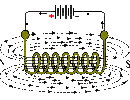
You should assume that the person reading the paper has taken PHYS 350 and has a knowledge of electromagnetism at the level of the class. In your paper, you should (1) introduce the topic, and explain the background to the problem and why it is interesting, (2) carefully describe (preferably with the help of a diagram or two) the basic physics of the process, device, or experiment, and (3) perform a simple calculation (at the “back of the envelope” level) which determines the basic quantities involved, and illustrates the physics. For example, you could describe the basic physics that causes a fridge magnet to stick to the metal door, and estimate the strength of the typical magnet needed, or describe the processes involved in a lightning strike, and estimate the charge transferred, typical currents, and frequency of lightning strikes around the globe.
PHYS350 Electromagnetism HELP(EXAM HELP, ONLINE TUTOR)
Show that the Green’s function for the 1-D Laplacian operator $\frac{d^2}{d x^2}$ is proportional to $\left|x-x^{\prime}\right|$. Find the proportionality constant. This could be useful in electrodynamics in a case where the charge density depends only on $x$ and not $y$ or $z$.
(a) Solve the $2 \mathrm{D}$ Laplace equation for the region $x \in[0, a], y \in[0, a]$ with boundary conditions that $V=0$ on all the sides except at $y=a$; there $V(x)=-E x$ for $x \leq a / 2$ and $-E(a-x)$ for $x \geq a / 2$. You may use Maple to do the integrals for the Fourier coefficients if you wish (and it would be a good idea to check your result with Maple even if you do it another way). (b) Use “plot3d” in Maple to plot the potential (use the “axes=boxed” option so that axes will be drawn), and verify that your solution obeys the boundary condition. How many terms in the Fourier series seem to be needed to get good convergence? How does the potential look when extended to the region $x \in[0,2 a]$ ? (c) Use “with(plots)” and “contourplot” to plot the equipotential surfaces. Sketch the result, and show also the electric field lines.
For a tutorial about solving this problem using Maple, see the other side. An electric dipole $\vec{p}$ with mass $m$ and moment of inertia $I$ starts out a distance $z_0$ along the $z$-axis above a point charge $Q$, with initial angle $\theta_0$ between $\vec{p}$ and $\vec{E}$. Assume it starts from rest. (a) Find the coupled equations of motion for $\theta$ and $z$. (b) Use Maple to numerically solve these equations and plot the solutions both $\theta(t)$ and $z(t))$ assuming that $p Q /\left4 \pi \epsilon_0 I\right=p Q /\left(2 \pi \epsilon_0 m\right=z_0=1$ in some units. Plot the solutions for $\theta_0$ close to 0 and to $\pi$ to show the different kinds of qualitative behavior. (c) By trial and error, find the critical value $\theta_c$ of $\theta_0$ such that the dipole just avoids crashing into the charge, to three significant figures. What curious behavior do the solutions display near this value? (d) Notice that for $\theta_0>\theta_c$, the ratio of rotational to translational energy approaches a constant at late times. Plot this ratio as a function of $\theta_0$, and find approximately the value of $\theta_0$ and the value of the ratio such that the latter is maximized. Although you could use Maple to find the rotational to translational energy as a function of $\theta_0$ and plot it directly, it may be faster for you to simply calculate it for a series of $\theta_0$ values and sketch the graph by hand.
Suppose you have solved the above problem for an abitrary potential $V_0(x)$ on the boundary at $y=a$, to get the potential $V(x, y)$. Show how the solution for the following problems can be expressed in terms of the above solution $V(x, y)$ : (a) $V=0$ on all boundaries except at $y=0$, where the value is $V_0(x)$; (b) $V=0$ at all boundaries except at $x=a$, where $V=V_0(y)$; (c) $V=V_0(y)$ at $x=0$ and vanishes at the other boundaries. (d) Using these results and the principle of superposition, find the solution for problem 1 when the function $V_0$ describes all four of the boundaries. Use Maple to plot $V$ again.
Do problem 5.15 , except assume there are 4 conductors, alternating between $V_0$ and $-V_0$, with the positive ones for $\phi \in[0, \pi / 2]$ and $[\pi, 3 \pi / 2]$, while the negative ones are at $\phi \in[\pi / 2, \pi],[3 \pi / 2,2 \pi]$. Make sure any coefficients of the Fourier series which vanish are so recognized. Hint: note that $\cos (n \pi)=(-1)^n$; show that $\sin (3 n \pi / 2)=(-1)^n \sin (n \pi / 2)$ and $\cos (3 n \pi / 2)=(-1)^n \cos (n \pi / 2)$.
Find the potential (for both $rR$ ) for the case where $V=V_0 \cos (\theta)^4$ on a spherical surface of radius $R$. Hint: $\cos (\theta)^4 \operatorname{can}$ be expressed as a linear combination of Legendre polynomials.

MY-ASSIGNMENTEXPERT™可以为您提供 CATALOG.YCP.EDU PHYS350 ELECTROMAGNETISM电磁学的代写代考和辅导服务!