如果你也在 怎样代写金融计量经济学Financial Econometrics 这个学科遇到相关的难题,请随时右上角联系我们的24/7代写客服。金融计量经济学Financial Econometrics是使用统计方法来发展理论或检验经济学或金融学的现有假设。计量经济学依靠的是回归模型和无效假设检验等技术。计量经济学也可用于尝试预测未来的经济或金融趋势。
金融计量经济学Financial Econometrics的一个基本工具是多元线性回归模型。计量经济学理论使用统计理论和数理统计来评估和发展计量经济学方法。计量经济学家试图找到具有理想统计特性的估计器,包括无偏性、效率和一致性。应用计量经济学使用理论计量经济学和现实世界的数据来评估经济理论,开发计量经济学模型,分析经济历史和预测。
金融计量经济学Financial Econometrics 免费提交作业要求, 满意后付款,成绩80\%以下全额退款,安全省心无顾虑。专业硕 博写手团队,所有订单可靠准时,保证 100% 原创。 最高质量的金融计量经济学Financial Econometrics作业代写,服务覆盖北美、欧洲、澳洲等 国家。 在代写价格方面,考虑到同学们的经济条件,在保障代写质量的前提下,我们为客户提供最合理的价格。 由于作业种类很多,同时其中的大部分作业在字数上都没有具体要求,因此金融计量经济学Financial Econometrics作业代写的价格不固定。通常在专家查看完作业要求之后会给出报价。作业难度和截止日期对价格也有很大的影响。
同学们在留学期间,都对各式各样的作业考试很是头疼,如果你无从下手,不如考虑my-assignmentexpert™!
my-assignmentexpert™提供最专业的一站式服务:Essay代写,Dissertation代写,Assignment代写,Paper代写,Proposal代写,Proposal代写,Literature Review代写,Online Course,Exam代考等等。my-assignmentexpert™专注为留学生提供Essay代写服务,拥有各个专业的博硕教师团队帮您代写,免费修改及辅导,保证成果完成的效率和质量。同时有多家检测平台帐号,包括Turnitin高级账户,检测论文不会留痕,写好后检测修改,放心可靠,经得起任何考验!
想知道您作业确定的价格吗? 免费下单以相关学科的专家能了解具体的要求之后在1-3个小时就提出价格。专家的 报价比上列的价格能便宜好几倍。
我们在经济Economy代写方面已经树立了自己的口碑, 保证靠谱, 高质且原创的经济Economy代写服务。我们的专家在微观经济学Microeconomics代写方面经验极为丰富,各种微观经济学Microeconomics相关的作业也就用不着 说。
经济代写|计量经济学代写Introduction to Econometrics代考|Time-Varying Betas
There is a large consensus in the literature about the fact that betas are actually timevarying. Such evidence has been pointed out by Fama and MacBeth (1973), Fabozzi and Francis (1977), Alexander and Chervany (1980), Sunder (1980), Ohlson and Rosenberg (1982), DeJong and Collins (1985), Fisher and Kamin (1985), Brooks et al. (1992), Brooks et al. (1994) among others. The aim of this section is therefore to review various methods used to estimate time-varying betas (and potentially timevarying alphas) in a conditional model close to Eq. (29):
$$
\tilde{r}{i, t}=\alpha_t+\sum{n=1}^N \beta_{n, t} \tilde{f}_{n, t}+\varepsilon_t,
$$
or equivalently (31):
$$
y_t=\mathbf{x}_t^{\prime} \boldsymbol{\beta}_t+\varepsilon_t
$$
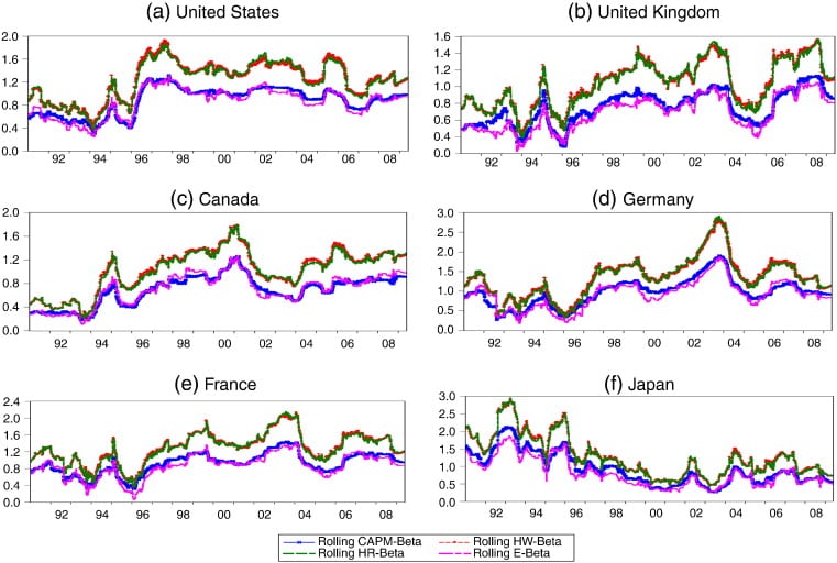
The first and simplest way to estimate time-varying betas is to estimate beta over moving sub-periods using a simple rolling-window OLS regression as proposed by Fama and MacBeth (1973) (see Van Nieuwerburgh 2019; Zhou 2013 for applications in the case of the REIT beta).
Let us assume we have historical data on a period spanning from $t_0$ to $t_T$. This method consists in selecting a window of $h$ observations (for instance 120 daily returns) and then estimating Eq. (30) by OLS over the first $h$ observations, that is from $t_0$ to $t_{0+h}$, so as to obtain $\left(\hat{\alpha}h, \hat{\beta}{1, h}, \ldots, \hat{\beta}{N, h}\right)^{\prime}$. Then, the window is rolled one step forward by adding one new observation and dropping the most distant one. So, $\left(\hat{\alpha}{h+1}, \hat{\beta}{1, h+1}, \ldots, \hat{\beta}{N, h+1}\right)^{\prime}$ are obtained in the same way over the period $t_{0+1}$ to $t_{0+h+1}$ and the sequence is reiterated until the end of the sample period.
This method can be considered as a quick and dirty time-varying regression model. When compared to the usual OLS regression model, the rolling-window OLS regression model offers the advantage of taking into account time variations in the alpha and the betas. However, the coefficients measured with this method only vary very slowly by construction due to the fact only one period is dropped and another is added between two successive estimates, which can lead to inaccurate estimates. The results also depend heavily on the size of the chosen window. ${ }^{16}$
经济代写|计量经济学代写Introduction to Econometrics代考|Realized Betas
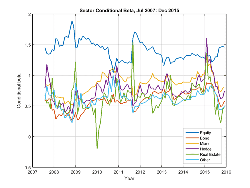
An alternative estimation method of time-varying betas is to compute both the realized variance and realized covariance from intraday ${ }^{17}$ data so as to estimate the beta using so called realized measures. The realized variance and covariance being computed from intraday data, they are much more accurate than standard measures (Hansen et al. 2014). This approach, based on the works of Andersen et al. (2003) and Barndorff-Nielsen and Shephard (2004), ${ }^{18}$ offers a more accurate way of analyzing the dynamic behavior of beta than the rolling beta methodology (Patton and Verardo 2012). In the context of a single factor model, the realized market beta, denoted $\beta^R$, is defined as
$$
\beta_t^R=\frac{\operatorname{cov}^R\left(\widetilde{r}i, \widetilde{r}_M\right)_t}{\operatorname{var}^R\left(\widetilde{r}_M\right)_t}=\frac{\sum{k=1}^{(s)} \tilde{r}(t){i, k} \widetilde{r}(t){M, k}}{\sum_{k=1}^{(s)} \widetilde{r}(t){M, k}^2}, $$ where $\operatorname{cov}^R\left(\widetilde{r}_i, \widetilde{r}_M\right)$ is the realized covariance between the asset’s excess return and the market excess return, $\left.\operatorname{and}{\operatorname{var}^R}{ }^R \widetilde{r}M\right)$ is the realized variance of the market excess return. $\tilde{r}(t){i, k}$ is the excess return on asset $i$ during the $k$ th intraday period on day $t$ and $s$ is the total number of intraday periods. ${ }^{19} \mathrm{As}$ a consequence, the realized beta is the ratio of an asset’s sample covariance with the market to the sample variance of the market over several intraday periods. ${ }^{20}$
This method resembles the rolling beta approach but it relies on non-overlapping windows (of one day or one month for instance) and requires data sampled at a higher frequency within each window (e.g., 5-minute returns). The main limit of this methodology is, therefore, the need for a sufficient number of intraday data in order to be able to compute the realized variance and covariance. See Boudt et al. (2017) for an extension to multi-factor betas.
计量经济学代写
经济代写|计量经济学代写Introduction to Econometrics代考|Time-Varying Betas
在文献中有一个很大的共识,即贝塔实际上是随时间变化的。Fama和MacBeth(1973)、Fabozzi和Francis(1977)、Alexander和Chervany(1980)、Sunder(1980)、Ohlson和Rosenberg(1982)、DeJong和Collins(1985)、Fisher和Kamin(1985)、Brooks et al.(1992)、Brooks et al.(1994)等人都指出了这些证据。因此,本节的目的是回顾在接近Eq.(29)的条件模型中用于估计时变beta(以及可能时变alpha)的各种方法:
$$
\tilde{r}{i, t}=\alpha_t+\sum{n=1}^N \beta_{n, t} \tilde{f}_{n, t}+\varepsilon_t,
$$
或等价(31):
$$
y_t=\mathbf{x}_t^{\prime} \boldsymbol{\beta}_t+\varepsilon_t
$$
估计时变贝塔的第一个也是最简单的方法是使用Fama和MacBeth(1973)提出的简单滚动窗口OLS回归来估计移动子周期的贝塔(参见Van Nieuwerburgh 2019;2013年周为申请情况下的REIT测试版)。
假设我们有从$t_0$到$t_T$这段时间的历史数据。这种方法是选择一个$h$观测值的窗口(例如120个日收益),然后对第一个$h$观测值,即从$t_0$到$t_{0+h}$,用OLS估计Eq.(30),从而得到$\left(\hat{\alpha}h, \hat{\beta}{1, h}, \ldots, \hat{\beta}{N, h}\right)^{\prime}$。然后,窗口向前滚动一步,增加一个新的观察结果,并放弃最远的观察结果。因此,在$t_{0+1}$到$t_{0+h+1}$期间以相同的方式获得$\left(\hat{\alpha}{h+1}, \hat{\beta}{1, h+1}, \ldots, \hat{\beta}{N, h+1}\right)^{\prime}$,并且重复该序列,直到样本周期结束。
这种方法可以看作是一种快速而肮脏的时变回归模型。与通常的OLS回归模型相比,滚动窗口OLS回归模型的优点是考虑了α和β的时间变化。然而,由于在两个连续的估计之间只删除一个周期,而另一个周期被添加,因此用这种方法测量的系数随构造的变化非常缓慢,这可能导致不准确的估计。结果也在很大程度上取决于所选窗口的大小。 ${ }^{16}$
经济代写|计量经济学代写Introduction to Econometrics代考|Realized Betas
时变贝塔的另一种估计方法是从当日${ }^{17}$数据中计算已实现方差和已实现协方差,从而使用所谓的已实现测度来估计贝塔。实现的方差和协方差是从日内数据中计算出来的,它们比标准测量要准确得多(Hansen et al. 2014)。这种方法基于Andersen等人(2003)和Barndorff-Nielsen和Shephard(2004)的作品,${ }^{18}$提供了一种比滚动beta方法更准确的分析beta动态行为的方法(Patton和Verardo 2012)。在单因素模型中,已实现的市场beta(记为$\beta^R$)定义为
$$
\beta_t^R=\frac{\operatorname{cov}^R\left(\widetilde{r}i, \widetilde{r}M\right)_t}{\operatorname{var}^R\left(\widetilde{r}_M\right)_t}=\frac{\sum{k=1}^{(s)} \tilde{r}(t){i, k} \widetilde{r}(t){M, k}}{\sum{k=1}^{(s)} \widetilde{r}(t){M, k}^2}, $$其中$\operatorname{cov}^R\left(\widetilde{r}_i, \widetilde{r}_M\right)$为资产超额收益与市场超额收益的已实现协方差,$\left.\operatorname{and}{\operatorname{var}^R}{ }^R \widetilde{r}M\right)$为市场超额收益的已实现方差。$\tilde{r}(t){i, k}$为$t$日$k$个日内期间资产$i$的超额收益,$s$为多个日内期间的总数。${ }^{19} \mathrm{As}$因此,已实现的贝塔是资产与市场的样本协方差与几个日内市场样本方差之比。 ${ }^{20}$
这种方法类似于滚动beta方法,但它依赖于不重叠的窗口(例如,一天或一个月),并且需要在每个窗口内以更高的频率采样数据(例如,5分钟的返回)。因此,这种方法的主要限制是需要足够数量的日内数据,以便能够计算已实现的方差和协方差。参见Boudt等人(2017)对多因素beta的扩展。

经济代写|计量经济学代考ECONOMETRICS代考 请认准UprivateTA™. UprivateTA™为您的留学生涯保驾护航。