如果你也在 怎样代写贝叶斯分析Bayesian Analysis 这个学科遇到相关的难题，请随时右上角联系我们的24/7代写客服。贝叶斯分析Bayesian Analysis是一种统计范式，它使用概率陈述来回答关于未知参数的研究问题。

贝叶斯分析Bayesian Analysis的独特特征包括能够将先验信息纳入分析，将可信区间直观地解释为固定范围，其中参数已知属于预先指定的概率，以及将实际概率分配给任何感兴趣的假设的能力。贝叶斯推断使用后验分布来形成模型参数的各种总结，包括点估计，如后验均值、中位数、百分位数和称为可信区间的区间估计。此外，所有关于模型参数的统计检验都可以表示为基于估计的后验分布的概率陈述。

同学们在留学期间，都对各式各样的作业考试很是头疼，如果你无从下手，不如考虑my-assignmentexpert™！

my-assignmentexpert™提供最专业的一站式服务：Essay代写，Dissertation代写，Assignment代写，Paper代写，Proposal代写，Proposal代写，Literature Review代写，Online Course，Exam代考等等。my-assignmentexpert™专注为留学生提供Essay代写服务，拥有各个专业的博硕教师团队帮您代写，免费修改及辅导，保证成果完成的效率和质量。同时有多家检测平台帐号，包括Turnitin高级账户，检测论文不会留痕，写好后检测修改，放心可靠，经得起任何考验！

统计代写|贝叶斯分析代考Bayesian Analysis代写|Posterior as compromise between data and prior information

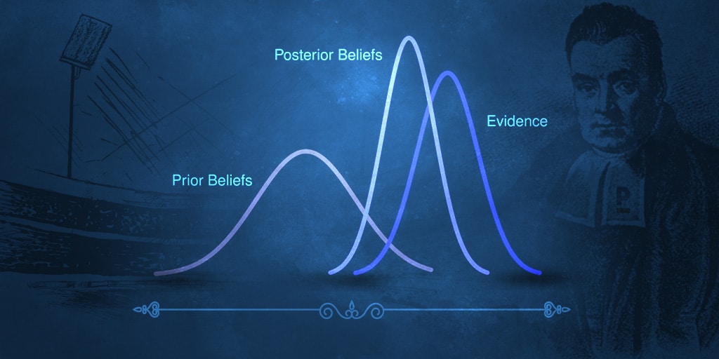
The process of Bayesian inference involves passing from a prior distribution, $p(\theta)$, to a posterior distribution, $p(\theta \mid y)$, and it is natural to expect that some general relations might hold between these two distributions. For example, we might expect that, because the posterior distribution incorporates the information from the data, it will be less variable than the prior distribution. This notion is formalized in the second of the following expressions:
$$
\mathrm{E}(\theta)=\mathrm{E}(\mathrm{E}(\theta \mid y))
$$
and
$$
\operatorname{var}(\theta)=\mathrm{E}(\operatorname{var}(\theta \mid y))+\operatorname{var}(\mathrm{E}(\theta \mid y)),
$$
which are obtained by substituting $(\theta, y)$ for the generic $(u, v)$ in (1.8) and (1.9). The result expressed by Equation (2.7) is scarcely surprising: the prior mean of $\theta$ is the average of all possible posterior means over the distribution of possible data. The variance formula (2.8) is more interesting because it says that the posterior variance is on average smaller than the prior variance, by an amount that depends on the variation in posterior means over the distribution of possible data. The greater the latter variation, the more the potential for reducing our uncertainty with regard to $\theta$, as we shall see in detail for the binomial and normal models in the next chapter. The mean and variance relations only describe expectations, and in particular situations the posterior variance can be similar to or even larger than the prior variance (although this can be an indication of conflict or inconsistency between the sampling model and prior distribution).

In the binomial example with the uniform prior distribution, the prior mean is $\frac{1}{2}$, and the prior variance is $\frac{1}{12}$. The posterior mean, $\frac{y+1}{n+2}$, is a compromise between the prior mean and the sample proportion, $\frac{y}{n}$, where clearly the prior mean has a smaller and smaller role as the size of the data sample increases. This is a general feature of Bayesian inference: the posterior distribution is centered at a point that represents a compromise between the prior information and the data, and the compromise is controlled to a greater extent by the data as the sample size increases.

统计代写|贝叶斯分析代考Bayesian Analysis代写|Summarizing posterior inference

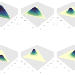
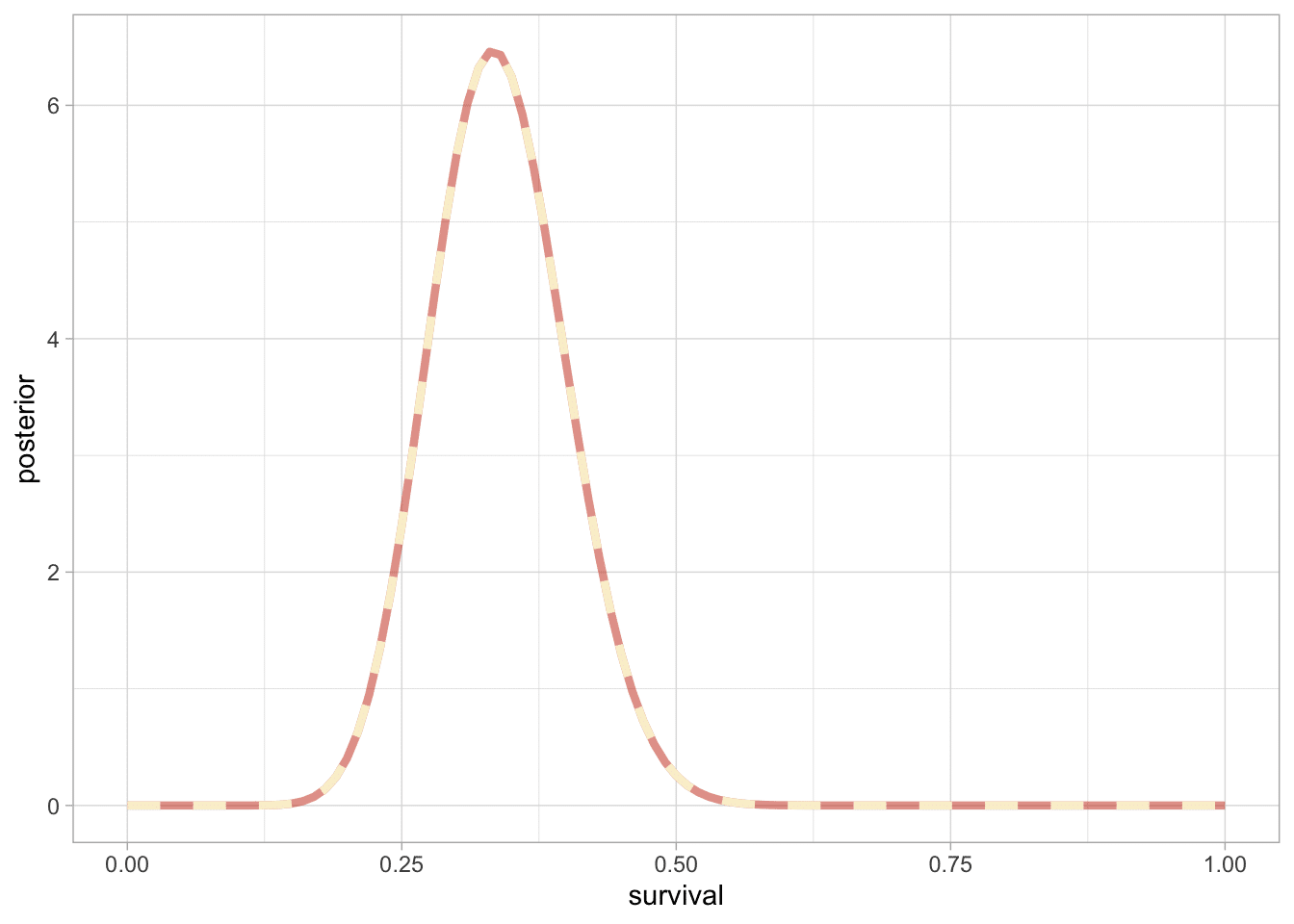
The posterior probability distribution contains all the current information about the parameter $\theta$. Ideally one might report the entire posterior distribution $p(\theta \mid y)$; as we have seen in Figure 2.1, a graphical display is useful. In Chapter 3, we use contour plots and scatterplots to display posterior distributions in multiparameter problems. A key advantage of the Bayesian approach, as implemented by simulation, is the flexibility with which posterior inferences can be summarized, even after complicated transformations. This advantage is most directly seen through examples, some of which will be presented shortly.

For many practical purposes, however, various numerical summaries of the distribution are desirable. Commonly used summaries of location are the mean, median, and mode(s) of the distribution; variation is commonly summarized by the standard deviation, the interquartile range, and other quantiles. Each summary has its own interpretation: for example, the mean is the posterior expectation of the parameter, and the mode may be interpreted as the single ‘most likely’ value, given the data (and the model). Furthermore, as we shall see, much practical inference relies on the use of normal approximations, often improved by applying a symmetrizing transformation to $\theta$, and here the mean and the standard deviation play key roles. The mode is important in computational strategies for more complex problems because it is often easier to compute than the mean or median.

When the posterior distribution has a closed form, such as the beta distribution in the current example, summaries such as the mean, median, and standard deviation of the posterior distribution are often available in closed form. For example, applying the distributional results in Appendix A, the mean of the beta distribution in (2.3) is $\frac{y+1}{n+2}$, and the mode is $\frac{y}{n}$, which is well known from different points of view as the maximum likelihood and (minimum variance) unbiased estimate of $\theta$.

贝叶斯分析代写

统计代写|贝叶斯分析代考Bayesian Analysis代写|Posterior as compromise between data and prior information

贝叶斯推理的过程涉及到从先验分布$p(\theta)$到后验分布$p(\theta \mid y)$，并且很自然地期望在这两个分布之间可能存在一些一般关系。例如，我们可能会期望，由于后验分布包含了来自数据的信息，因此它将比先验分布的变量更少。这个概念可以用下列第二种形式来形式化:
$$
\mathrm{E}(\theta)=\mathrm{E}(\mathrm{E}(\theta \mid y))
$$
和
$$
\operatorname{var}(\theta)=\mathrm{E}(\operatorname{var}(\theta \mid y))+\operatorname{var}(\mathrm{E}(\theta \mid y)),
$$
通过将(1.8)和式(1.9)中的通用$(u, v)$替换为$(\theta, y)$得到。公式(2.7)表示的结果并不令人惊讶:$\theta$的先验均值是所有可能的后验均值在可能数据分布上的平均值。方差公式(2.8)更有趣，因为它表示后验方差平均小于先验方差，其大小取决于后验均值在可能数据分布上的变化。后一种变化越大，就越有可能减少我们关于$\theta$的不确定性，我们将在下一章中详细讨论二项和正态模型。均值和方差关系仅描述期望，在特定情况下，后验方差可能与先验方差相似甚至大于先验方差(尽管这可能表明抽样模型与先验分布之间存在冲突或不一致)。

在均匀先验分布的二项示例中，先验均值为$\frac{1}{2}$，先验方差为$\frac{1}{12}$。后验均值$\frac{y+1}{n+2}$是先验均值和样本比例$\frac{y}{n}$之间的一个折衷，显然，随着数据样本规模的增加，先验均值的作用越来越小。这是贝叶斯推理的一个普遍特征:后验分布的中心在一个点上，这个点代表了先验信息和数据之间的妥协，并且随着样本量的增加，这种妥协在更大程度上受到数据的控制。

统计代写|贝叶斯分析代考Bayesian Analysis代写|Summarizing posterior inference

后验概率分布包含了关于$\theta$参数的所有当前信息。理想情况下可以报告整个后验分布$p(\theta \mid y)$;如图2.1所示，图形显示非常有用。在第三章中，我们使用等高线图和散点图来显示多参数问题的后验分布。通过仿真实现的贝叶斯方法的一个关键优势是，即使在复杂的转换之后，也可以灵活地总结后验推断。这种优势可以通过示例最直接地看到，稍后将介绍其中的一些示例。

然而，对于许多实际用途，需要对分布进行各种数值总结。常用的位置摘要是分布的平均值、中位数和众数;变异通常用标准差、四分位数间距和其他分位数来概括。每个摘要都有自己的解释:例如，均值是参数的后验期望，而模态可能被解释为给定数据(和模型)的单个“最可能”值。此外，正如我们将看到的，许多实际推断依赖于正态近似的使用，通常通过对$\theta$应用对称变换来改进，这里的平均值和标准差起着关键作用。该模型在复杂问题的计算策略中很重要，因为它通常比平均值或中位数更容易计算。

当后验分布具有封闭形式时，例如本例中的beta分布，后验分布的均值、中位数和标准差等摘要通常以封闭形式提供。例如，应用附录A中的分布结果，(2.3)中beta分布的均值为$\frac{y+1}{n+2}$，众数为$\frac{y}{n}$，从不同的角度来看，它被称为$\theta$的最大似然和(最小方差)无偏估计。

统计代写|贝叶斯分析代考Bayesian Analysis代写 请认准exambang™. exambang™为您的留学生涯保驾护航。

微观经济学代写

微观经济学是主流经济学的一个分支，研究个人和企业在做出有关稀缺资源分配的决策时的行为以及这些个人和企业之间的相互作用。my-assignmentexpert™ 为您的留学生涯保驾护航 在数学Mathematics作业代写方面已经树立了自己的口碑, 保证靠谱, 高质且原创的数学Mathematics代写服务。我们的专家在图论代写Graph Theory代写方面经验极为丰富，各种图论代写Graph Theory相关的作业也就用不着 说。

线性代数代写

线性代数是数学的一个分支，涉及线性方程，如：线性图，如：以及它们在向量空间和通过矩阵的表示。线性代数是几乎所有数学领域的核心。

博弈论代写

现代博弈论始于约翰-冯-诺伊曼（John von Neumann）提出的两人零和博弈中的混合策略均衡的观点及其证明。冯-诺依曼的原始证明使用了关于连续映射到紧凑凸集的布劳威尔定点定理，这成为博弈论和数学经济学的标准方法。在他的论文之后，1944年，他与奥斯卡-莫根斯特恩（Oskar Morgenstern）共同撰写了《游戏和经济行为理论》一书，该书考虑了几个参与者的合作游戏。这本书的第二版提供了预期效用的公理理论，使数理统计学家和经济学家能够处理不确定性下的决策。

微积分代写

微积分，最初被称为无穷小微积分或 “无穷小的微积分”，是对连续变化的数学研究，就像几何学是对形状的研究，而代数是对算术运算的概括研究一样。

它有两个主要分支，微分和积分；微分涉及瞬时变化率和曲线的斜率，而积分涉及数量的累积，以及曲线下或曲线之间的面积。这两个分支通过微积分的基本定理相互联系，它们利用了无限序列和无限级数收敛到一个明确定义的极限的基本概念 。

计量经济学代写

什么是计量经济学？
计量经济学是统计学和数学模型的定量应用，使用数据来发展理论或测试经济学中的现有假设，并根据历史数据预测未来趋势。它对现实世界的数据进行统计试验，然后将结果与被测试的理论进行比较和对比。

根据你是对测试现有理论感兴趣，还是对利用现有数据在这些观察的基础上提出新的假设感兴趣，计量经济学可以细分为两大类：理论和应用。那些经常从事这种实践的人通常被称为计量经济学家。

Matlab代写

MATLAB 是一种用于技术计算的高性能语言。它将计算、可视化和编程集成在一个易于使用的环境中，其中问题和解决方案以熟悉的数学符号表示。典型用途包括：数学和计算算法开发建模、仿真和原型制作数据分析、探索和可视化科学和工程图形应用程序开发，包括图形用户界面构建MATLAB 是一个交互式系统，其基本数据元素是一个不需要维度的数组。这使您可以解决许多技术计算问题，尤其是那些具有矩阵和向量公式的问题，而只需用 C 或 Fortran 等标量非交互式语言编写程序所需的时间的一小部分。MATLAB 名称代表矩阵实验室。MATLAB 最初的编写目的是提供对由 LINPACK 和 EISPACK 项目开发的矩阵软件的轻松访问，这两个项目共同代表了矩阵计算软件的最新技术。MATLAB 经过多年的发展，得到了许多用户的投入。在大学环境中，它是数学、工程和科学入门和高级课程的标准教学工具。在工业领域，MATLAB 是高效研究、开发和分析的首选工具。MATLAB 具有一系列称为工具箱的特定于应用程序的解决方案。对于大多数 MATLAB 用户来说非常重要，工具箱允许您学习和应用专业技术。工具箱是 MATLAB 函数（M 文件）的综合集合，可扩展 MATLAB 环境以解决特定类别的问题。可用工具箱的领域包括信号处理、控制系统、神经网络、模糊逻辑、小波、仿真等。