0 0

By admin 生存模型统计统计代写 2023年8月7日

代写隐藏

1 统计代写|生存模型代考Survival Models代写|Non-Parametric Estimation

2 统计代写|生存模型代考Survival Models代写|Parametric Estimation

3.1 统计代写|生存模型代考Survival Models代写|Non-Parametric Estimation

3.2 统计代写|生存模型代考Survival Models代写|Parametric Estimation

如果你也在怎样代写生存模型Survival Models这个学科遇到相关的难题，请随时右上角联系我们的24/7代写客服。生存模型Survival Models在许多可用于分析事件时间数据的模型中，有4个是最突出的:Kaplan Meier模型、指数模型、Weibull模型和Cox比例风险模型。

生存模型Survival Models精算师和其他应用数学家使用预测人类或其他实体(有生命或无生命)生存模式的模型，并经常使用这些模型作为相当重要的财务计算的基础。具体来说，精算师使用这些模型来计算与个人人寿保险单、养老金计划和收入损失保险相关的财务价值。人口统计学家和其他社会科学家使用生存模型对该模型适用的人口的未来构成做出预测。

生存模型Survival Models代写，免费提交作业要求，满意后付款，成绩80\%以下全额退款，安全省心无顾虑。专业硕博写手团队，所有订单可靠准时，保证 100% 原创。最高质量的生存模型Survival Models作业代写，服务覆盖北美、欧洲、澳洲等国家。在代写价格方面，考虑到同学们的经济条件，在保障代写质量的前提下，我们为客户提供最合理的价格。由于作业种类很多，同时其中的大部分作业在字数上都没有具体要求，因此生存模型Survival Models作业代写的价格不固定。通常在专家查看完作业要求之后会给出报价。作业难度和截止日期对价格也有很大的影响。

同学们在留学期间，都对各式各样的作业考试很是头疼，如果你无从下手，不如考虑my-assignmentexpert™！

my-assignmentexpert™提供最专业的一站式服务：Essay代写，Dissertation代写，Assignment代写，Paper代写，Proposal代写，Proposal代写，Literature Review代写，Online Course，Exam代考等等。my-assignmentexpert™专注为留学生提供Essay代写服务，拥有各个专业的博硕教师团队帮您代写，免费修改及辅导，保证成果完成的效率和质量。同时有多家检测平台帐号，包括Turnitin高级账户，检测论文不会留痕，写好后检测修改，放心可靠，经得起任何考验！

统计代写|生存模型代考Survival Models代写|Non-Parametric Estimation

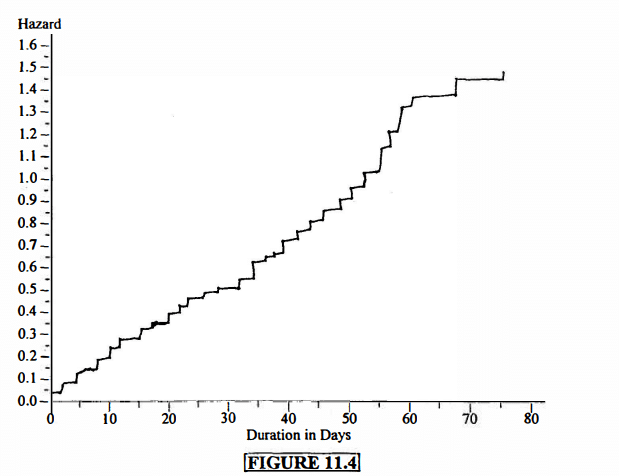
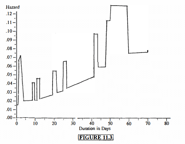
The data given in Table 11.1, taken from Kennan [45], show lengths of strikes in U.S. manufacturing industries over the period from 1968 to 1976. To achieve a degree of homogeneity, only official strikes involving 1000 or more workers, in which the major issue was general wage changes as classified by the Bureau of Labor Statistics, are included. Furthermore, only strikes beginning in June of each year in the study period are considered to avoid seasonal heterogeneity. There are 62 total strikes in the data set.

There are 12 strikes in the data set whose lengths were rightcensored at 80 days. There are also several ties in the data, with 4 strikes lasting 2 days, another 4 lasting 3 days, and so on.

For each ordered duration $j$, let $t_j$ denote the length of that duration and let $d_j$ denote the number of strikes lasting exactly $t_j$ days, so that $d_j$ represents the number of strike terminations at time $t_j$. Let $r_j$ denote the risk set of strikes still in effect just before time $t_j$. Then the conditional probability of ending a strike at duration $t_j$, given that it has reached duration $t_j$, is estimated by
$$
\hat{q}j=\frac{d_j}{r_j} . $$ The literature dealing with the duration of economic events tends to refer to this conditional (discrete) probability as a hazard function, although in this text we tend to restrict the term hazard function to the continuous case. Then we can also write $$ \hat{\lambda}\left(t_j\right)=\frac{d_j}{r_j} . $$ The natural estimator for the survival function is the Kaplan-Meier (or product-limit) estimator, developed in Section 7.6, which is $$ \hat{S}\left(t_j\right)=\prod{i=1}^j\left(\frac{r_i-d_i}{r_i}\right)
$$

统计代写|生存模型代考Survival Models代写|Parametric Estimation

The parameters of a distribution can be estimated by maximum likelihood. If we have full data, then the likelihood function is
$$
L(\theta)=\prod_{j=1}^n f\left(\boldsymbol{t}j ; \boldsymbol{\theta}\right), $$ where $\theta$ is a vector of one or more parameters and $f\left(t_j ; \theta\right)$ denotes the PDF at the $j^{\text {th }}$ duration. When the data are censored, as with the strike data, the contribution to likelihood of a censored observation is the SDF evaluated at the censored duration, which is 80 in this case. We define the indicator variable $\delta_j$ to be $\delta_j=1$ if the end of the strike is observed (i.e., not censored) and $\delta_j=0$ if the $j^{t h}$ observation has been censored. Then the likelihood is $$ L(\theta)=\prod{j=1}^n\left[f\left(t_j ; \theta\right)\right]^{\delta_j} \cdot\left[S\left(t_j ; \theta\right)\right]^{1-\delta_j}
$$

and the log-likelihood is
$$
\ell(\theta)=\sum_{j=1}^n \delta_j \cdot \ln \left[f\left(t_j ; \theta\right)\right]+\sum_{j=1}^n\left(1-\delta_j\right) \cdot \ln \left[S\left(t_j ; \theta\right)\right] .
$$
Substituting $f\left(t_j ; \theta\right)=S\left(t_j ; \theta\right) \cdot \lambda\left(t_j ; \theta\right)$, we have
$$
\ell(\theta)=\sum_{j=1}^n \ln \left[S\left(t_j ; \theta\right)\right]+\sum_{j=1}^n \delta_j \cdot \ln \left[\lambda\left(t_j ; \theta\right)\right]
$$
If we select the exponential distribution as our model for the strike data, we have the well-known result
$$
\hat{\theta}=\hat{\lambda}=\frac{\sum_{j=1}^n \delta_j}{\sum_{j=1}^n t_j},
$$
as derived in Chapter 8 (see Section 8.2), where $\sum_{j=1}^n \delta_j$ is the number of observed strike endings and $\sum_{j=1}^n t_j$ is the exact exposure of being on strike. From the data in Table 11.1 we calculate $\sum_{j=1}^{62} t_j=2118$ and $\sum_{j=1}^{62} \delta_J=50$, giving us $\hat{\lambda}=\frac{50}{21{ }^1}=.0236$.

生存模型代考

统计代写|生存模型代考Survival Models代写|Non-Parametric Estimation

表11.1给出的数据来自Kennan[45]，显示了1968年至1976年期间美国制造业罢工的时长。为了达到一定程度的同质性，只有涉及1000名或以上工人的官方罢工，其中主要问题是劳工统计局分类的一般工资变化，才被包括在内。此外，仅考虑研究期间每年6月开始的罢工，以避免季节性异质性。数据集中总共有62次罢工。

数据集中有12次罢工，其长度被正确审查为80天。数据中也有几个平手，4次击球持续2天，另外4次击球持续3天，以此类推。

对于每个订购的持续时间$j$，让$t_j$表示该持续时间的长度，让$d_j$表示持续时间正好为$t_j$天的罢工次数，因此$d_j$表示在$t_j$时间终止罢工的次数。让$r_j$表示在$t_j$时间之前仍然有效的罢工的风险集。然后，在罢工持续时间$t_j$结束罢工的条件概率，假设罢工持续时间$t_j$，估计为
$$
\hat{q}j=\frac{d_j}{r_j} . $$处理经济事件持续时间的文献倾向于将这种条件(离散)概率称为风险函数，尽管在本文中，我们倾向于将术语风险函数限制为连续情况。然后我们也可以写$$ \hat{\lambda}\left(t_j\right)=\frac{d_j}{r_j} . $$生存函数的自然估计量是Kaplan-Meier(或product-limit)估计量，在7.6节中开发，它是 $$ \hat{S}\left(t_j\right)=\prod{i=1}^j\left(\frac{r_i-d_i}{r_i}\right)
$$

统计代写|生存模型代考Survival Models代写|Parametric Estimation

分布的参数可以用最大似然估计。如果我们有完整的数据，那么似然函数是
$$
L(\theta)=\prod_{j=1}^n f\left(\boldsymbol{t}j ; \boldsymbol{\theta}\right), $$其中$\theta$是一个或多个参数的矢量，$f\left(t_j ; \theta\right)$表示$j^{\text {th }}$持续时间的PDF。当数据被审查时，与罢工数据一样，对审查观测的可能性的贡献是在审查持续时间内评估的SDF，在这种情况下为80。如果观察到罢工的结束(即未被审查)，我们将指标变量$\delta_j$定义为$\delta_j=1$，如果观察到$j^{t h}$已被审查，则将其定义为$\delta_j=0$。那么可能性是 $$ L(\theta)=\prod{j=1}^n\left[f\left(t_j ; \theta\right)\right]^{\delta_j} \cdot\left[S\left(t_j ; \theta\right)\right]^{1-\delta_j}
$$

对数似然是
$$
\ell(\theta)=\sum_{j=1}^n \delta_j \cdot \ln \left[f\left(t_j ; \theta\right)\right]+\sum_{j=1}^n\left(1-\delta_j\right) \cdot \ln \left[S\left(t_j ; \theta\right)\right] .
$$
代入$f\left(t_j ; \theta\right)=S\left(t_j ; \theta\right) \cdot \lambda\left(t_j ; \theta\right)$，得到
$$
\ell(\theta)=\sum_{j=1}^n \ln \left[S\left(t_j ; \theta\right)\right]+\sum_{j=1}^n \delta_j \cdot \ln \left[\lambda\left(t_j ; \theta\right)\right]
$$
如果我们选择指数分布作为我们的走向数据模型，我们有众所周知的结果
$$
\hat{\theta}=\hat{\lambda}=\frac{\sum_{j=1}^n \delta_j}{\sum_{j=1}^n t_j},
$$
由第8章(参见8.2节)推导而来，其中$\sum_{j=1}^n \delta_j$是观察到的罢工结束次数，$\sum_{j=1}^n t_j$是罢工的确切暴露次数。根据表11.1中的数据，我们计算$\sum_{j=1}^{62} t_j=2118$和$\sum_{j=1}^{62} \delta_J=50$，得到$\hat{\lambda}=\frac{50}{21{ }^1}=.0236$。