如果你也在 怎样代写信息论information theory 这个学科遇到相关的难题,请随时右上角联系我们的24/7代写客服。信息论information theory回答了通信理论中的两个基本问题:什么是最终的数据压缩(答案:熵$H$),什么是通信的最终传输速率(答案:信道容量$C$)。由于这个原因,一些人认为信息论是通信理论的一个子集。我们认为它远不止于此。
信息论information theory在统计物理学(热力学)、计算机科学(柯尔莫哥洛夫复杂性或算法复杂性)、统计推断(奥卡姆剃刀:“最简单的解释是最好的”)以及概率和统计学(最优假设检验和估计的误差指数)方面都做出了根本性的贡献。
my-assignmentexpert™信息论information theory代写,免费提交作业要求, 满意后付款,成绩80\%以下全额退款,安全省心无顾虑。专业硕 博写手团队,所有订单可靠准时,保证 100% 原创。my-assignmentexpert, 最高质量的信息论information theory作业代写,服务覆盖北美、欧洲、澳洲等 国家。 在代写价格方面,考虑到同学们的经济条件,在保障代写质量的前提下,我们为客户提供最合理的价格。 由于统计Statistics作业种类很多,同时其中的大部分作业在字数上都没有具体要求,因此信息论information theory作业代写的价格不固定。通常在经济学专家查看完作业要求之后会给出报价。作业难度和截止日期对价格也有很大的影响。
想知道您作业确定的价格吗? 免费下单以相关学科的专家能了解具体的要求之后在1-3个小时就提出价格。专家的 报价比上列的价格能便宜好几倍。
my-assignmentexpert™ 为您的留学生涯保驾护航 在澳洲代写方面已经树立了自己的口碑, 保证靠谱, 高质且原创的澳洲代写服务。我们的专家在信息论information theory代写方面经验极为丰富,各种信息论information theory相关的作业也就用不着 说。
数学代写|信息论代写Information Theory代考|First Step: The Locational SMI of a Particle in a $1 D$ Box of Length $\mathrm{L}$
Figure 2.1 a shows a particle confined to a one-dimensional (1D) “box” of length $L$. The corresponding continuous SMI is:
$$
H[f(x)]=-\int f(x) \log f(x) d x
$$
Note that in Eq. (2.1), the SMI (denote $H$ ) is viewed as a functional of the function $f(x)$, where $f(x) d x$ is the probability of finding the particle in an interval between $x$ an $x+d x$.
Next, calculate the specific density distribution which maximizes the locational SMI, in (2.1). It is easy to show that the result is (see reference [1]):
$$
f_{e q}(x)=\frac{1}{L}
$$
Since we know that the probability of finding the particle at any interval is $1 / \mathrm{L}$, we may identify the distribution which maximizes the SMI as the equilibrium (eq.) distribution. The justification for this is explained in details in Ben-Naim [1, 4]. From (2.2) in (2.1) we obtain the maximum value of the SMI over all possible locational distribution:
$$
H(\text { locations in } 1 D)=\log L
$$
Next we admit that the location of the particle cannot be determined with absolute accuracy; there exists a small interval $h_x$ within which we do not care where the particle is. Therefore, we must correct Eq. (2.3) by subtracting $\log h_x$. Thus, we write instead of (2.3), the modified $H$ (locations in 1D) as:
$$
H\left(\text { locations in 1D) }=\log L-\log h_x\right.
$$
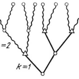
In the last equation we effectively defined $H$ (locations in 1D) for the finite number of intervals $n=L / h$. The passage from the infinite to the finite case is shown in Fig. 2.1b. Note that when $h_x \rightarrow 0, H$ (locations in 1D) diverges to infinity. Here, we do not take the strict mathematical limit, but we stop at $h_x$ which is small enough, but not zero. Note also that the ratio of $L$ and $h_x$ is a pure number. Hence we do not need to specify the units of either $L$ or $h_x$.
数学代写|信息论代写Information Theory代考|Second Step: The Velocity SMI of a Particle in a $1 D$ “Box” of Length $\mathrm{L}$
In the second step we calculate the probability distribution that maximizes the (continuous) SMI, subject to two conditions:
$$
\begin{gathered}
\int_{-\infty}^{\infty} f(x) d x=1 \
\int_{-\infty}^{\infty} x^2 f(x) d x=\sigma^2=\text { constant }
\end{gathered}
$$
In his original paper, Shannon [5] proved that the function $f(x)$ which maximize the SMI in (2.1), subject to the two conditions (2.5) and (2.6), is the Normal distribution, i.e.:
$$
f_{e q}(x)=\frac{\exp \left[-x^2 / 2 \sigma^2\right]}{\sqrt{2 \pi \sigma^2}}
$$
Note again that we use the subscript eq. for equilibrium. Applying this result to a classical particle having average kinetic energy $\frac{\left.m<v_x^2\right\rangle}{2}$, and using the relationship between the standard deviation $\sigma^2$ and the temperature of the system:
$$
\sigma^2=\frac{k_B T}{m}
$$
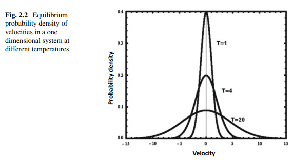
we obtain the equilibrium velocity distribution of one particle in a $1 \mathrm{D}$ system. This is shown in Fig. 2.2:
$$
f_{e q}\left(v_x\right)=\sqrt{\frac{m}{2 \pi k_B T}} \exp \left[\frac{-m v_x^2}{2 k_B T}\right]
$$
Here, $k_B$ is the Boltzmann constant, $m$ is the mass of the particle, and $T$ the absolute temperature.
The value of the (continuous) SMI for this probability density is:
$$
H_{\max }(\text { velocity in } 1 D)=\frac{1}{2} \log \left(2 \pi e k_B T / m\right)
$$
信息论代写
数学代写|信息论代写Information Theory代考|First Step: The Locational SMI of a Particle in a $1 D$ Box of Length $\mathrm{L}$
图2.1 a显示了一个局限于一维(1D)的粒子。长度为$L$的“盒子”。对应的连续SMI为:
$$
H[f(x)]=-\int f(x) \log f(x) d x
$$
注意,在Eq.(2.1)中,SMI(表示$H$)被视为函数$f(x)$的函数,其中$f(x) d x$是在$x$和$x+d x$之间的区间内找到粒子的概率。
接下来,计算使位置SMI最大化的比密度分布,见(2.1)。结果很容易证明(参见文献[1]):
$$
f_{e q}(x)=\frac{1}{L}
$$
由于我们知道在任何间隔找到粒子的概率为$1 / \mathrm{L}$,我们可以将SMI最大化的分布确定为平衡(eq.)分布。对此,Ben-Naim[1,4]中有详细的解释。由式(2.2)和式(2.1)可以得到SMI在所有可能的位置分布上的最大值:
$$
H(\text { locations in } 1 D)=\log L
$$
其次,我们承认不能绝对精确地确定粒子的位置;存在一个小的区间$h_x$在这个区间内我们不关心粒子在哪里。因此,我们必须通过减去$\log h_x$来修正Eq.(2.3)。因此,我们将修改后的$H$ (locations in 1D)写成(2.3):
$$
H\left(\text { locations in 1D) }=\log L-\log h_x\right.
$$
在上一个方程中,我们有效地为有限数量的区间$n=L / h$定义了$H$ (1D中的位置)。从无限到有限的过渡如图2.1b所示。注意,当$h_x \rightarrow 0, H$ (1D中的位置)发散到无穷大时。这里,我们不取严格的数学极限,但我们停在$h_x$,它足够小,但不是零。还要注意$L$和$h_x$的比率是一个纯数字。因此,我们不需要指定$L$或$h_x$的单位。
数学代写|信息论代写Information Theory代考|Second Step: The Velocity SMI of a Particle in a $1 D$ “Box” of Length $\mathrm{L}$
在第二步中,我们计算(连续)SMI最大化的概率分布,需要满足两个条件:
$$
\begin{gathered}
\int_{-\infty}^{\infty} f(x) d x=1 \
\int_{-\infty}^{\infty} x^2 f(x) d x=\sigma^2=\text { constant }
\end{gathered}
$$
Shannon[5]在其原始论文中证明了(2.1)中SMI最大的函数$f(x)$在满足(2.5)和式(2.6)两个条件下为正态分布,即:
$$
f_{e q}(x)=\frac{\exp \left[-x^2 / 2 \sigma^2\right]}{\sqrt{2 \pi \sigma^2}}
$$
再次注意,我们用下标等式表示平衡。将此结果应用于具有平均动能$\frac{\left.m<v_x^2\right\rangle}{2}$的经典粒子,并利用标准偏差$\sigma^2$与系统温度之间的关系:
$$
\sigma^2=\frac{k_B T}{m}
$$
我们得到了$1 \mathrm{D}$系统中一个粒子的平衡速度分布。如图2.2所示:
$$
f_{e q}\left(v_x\right)=\sqrt{\frac{m}{2 \pi k_B T}} \exp \left[\frac{-m v_x^2}{2 k_B T}\right]
$$
这里,$k_B$是玻尔兹曼常数,$m$是粒子的质量,$T$是绝对温度。
该概率密度的(连续)SMI值为:
$$
H_{\max }(\text { velocity in } 1 D)=\frac{1}{2} \log \left(2 \pi e k_B T / m\right)
$$

数学代写|信息论代写Information Theory代考 请认准UprivateTA™. UprivateTA™为您的留学生涯保驾护航。
微观经济学代写
微观经济学是主流经济学的一个分支,研究个人和企业在做出有关稀缺资源分配的决策时的行为以及这些个人和企业之间的相互作用。my-assignmentexpert™ 为您的留学生涯保驾护航 在数学Mathematics作业代写方面已经树立了自己的口碑, 保证靠谱, 高质且原创的数学Mathematics代写服务。我们的专家在图论代写Graph Theory代写方面经验极为丰富,各种图论代写Graph Theory相关的作业也就用不着 说。
线性代数代写
线性代数是数学的一个分支,涉及线性方程,如:线性图,如:以及它们在向量空间和通过矩阵的表示。线性代数是几乎所有数学领域的核心。
博弈论代写
现代博弈论始于约翰-冯-诺伊曼(John von Neumann)提出的两人零和博弈中的混合策略均衡的观点及其证明。冯-诺依曼的原始证明使用了关于连续映射到紧凑凸集的布劳威尔定点定理,这成为博弈论和数学经济学的标准方法。在他的论文之后,1944年,他与奥斯卡-莫根斯特恩(Oskar Morgenstern)共同撰写了《游戏和经济行为理论》一书,该书考虑了几个参与者的合作游戏。这本书的第二版提供了预期效用的公理理论,使数理统计学家和经济学家能够处理不确定性下的决策。
微积分代写
微积分,最初被称为无穷小微积分或 “无穷小的微积分”,是对连续变化的数学研究,就像几何学是对形状的研究,而代数是对算术运算的概括研究一样。
它有两个主要分支,微分和积分;微分涉及瞬时变化率和曲线的斜率,而积分涉及数量的累积,以及曲线下或曲线之间的面积。这两个分支通过微积分的基本定理相互联系,它们利用了无限序列和无限级数收敛到一个明确定义的极限的基本概念 。
计量经济学代写
什么是计量经济学?
计量经济学是统计学和数学模型的定量应用,使用数据来发展理论或测试经济学中的现有假设,并根据历史数据预测未来趋势。它对现实世界的数据进行统计试验,然后将结果与被测试的理论进行比较和对比。
根据你是对测试现有理论感兴趣,还是对利用现有数据在这些观察的基础上提出新的假设感兴趣,计量经济学可以细分为两大类:理论和应用。那些经常从事这种实践的人通常被称为计量经济学家。
Matlab代写
MATLAB 是一种用于技术计算的高性能语言。它将计算、可视化和编程集成在一个易于使用的环境中,其中问题和解决方案以熟悉的数学符号表示。典型用途包括:数学和计算算法开发建模、仿真和原型制作数据分析、探索和可视化科学和工程图形应用程序开发,包括图形用户界面构建MATLAB 是一个交互式系统,其基本数据元素是一个不需要维度的数组。这使您可以解决许多技术计算问题,尤其是那些具有矩阵和向量公式的问题,而只需用 C 或 Fortran 等标量非交互式语言编写程序所需的时间的一小部分。MATLAB 名称代表矩阵实验室。MATLAB 最初的编写目的是提供对由 LINPACK 和 EISPACK 项目开发的矩阵软件的轻松访问,这两个项目共同代表了矩阵计算软件的最新技术。MATLAB 经过多年的发展,得到了许多用户的投入。在大学环境中,它是数学、工程和科学入门和高级课程的标准教学工具。在工业领域,MATLAB 是高效研究、开发和分析的首选工具。MATLAB 具有一系列称为工具箱的特定于应用程序的解决方案。对于大多数 MATLAB 用户来说非常重要,工具箱允许您学习和应用专业技术。工具箱是 MATLAB 函数(M 文件)的综合集合,可扩展 MATLAB 环境以解决特定类别的问题。可用工具箱的领域包括信号处理、控制系统、神经网络、模糊逻辑、小波、仿真等。