电子工程代写|电路设计作业代写Intro to circuit design代考|Classification and Regression Model

如果你也在 怎样代写电路设计Intro to circuit design这个学科遇到相关的难题，请随时右上角联系我们的24/7代写客服。电路设计Intro to circuit design一个简单的电路由电阻器、电容器、电感器、晶体管、二极管和集成电路组成。这些基本的电子元件是由导电线连接的。电流可以很容易地在这些导线之间流动，以便使电子元件处于工作状态。

电路设计Intro to circuit design过程从规格书开始，规格书说明了成品设计必须提供的功能，但没有指出如何实现这些功能。最初的规格书基本上是对客户希望成品电路实现的技术上的详细描述，可以包括各种电气要求，如电路将接收什么信号，必须输出什么信号，有什么电源，允许消耗多少功率。规格书还可以（通常也是如此）设定设计必须满足的一些物理参数，如尺寸、重量、防潮性、温度范围、热输出、振动容限和加速度容限等。

my-assignmentexpert™ 电路设计Intro to circuit design作业代写，免费提交作业要求， 满意后付款，成绩80\%以下全额退款，安全省心无顾虑。专业硕 博写手团队，所有订单可靠准时，保证 100% 原创。my-assignmentexpert™， 最高质量的电路设计Intro to circuit design作业代写，服务覆盖北美、欧洲、澳洲等 国家。 在代写价格方面，考虑到同学们的经济条件，在保障代写质量的前提下，我们为客户提供最合理的价格。 由于统计Statistics作业种类很多，同时其中的大部分作业在字数上都没有具体要求，因此电路设计Intro to circuit design作业代写的价格不固定。通常在经济学专家查看完作业要求之后会给出报价。作业难度和截止日期对价格也有很大的影响。

想知道您作业确定的价格吗? 免费下单以相关学科的专家能了解具体的要求之后在1-3个小时就提出价格。专家的 报价比上列的价格能便宜好几倍。

my-assignmentexpert™ 为您的留学生涯保驾护航 在电子工程Electrical Engineering作业代写方面已经树立了自己的口碑, 保证靠谱, 高质且原创的电子工程Electrical Engineering代写服务。我们的专家在电路设计Intro to circuit design代写方面经验极为丰富，各种电路设计Intro to circuit design相关的作业也就用不着 说。

我们提供的电路设计Intro to circuit design及其相关学科的代写，服务范围广, 其中包括但不限于:

电子工程代写|电路设计作业代写Intro to circuit design代考|Classification and Regression Model

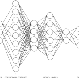
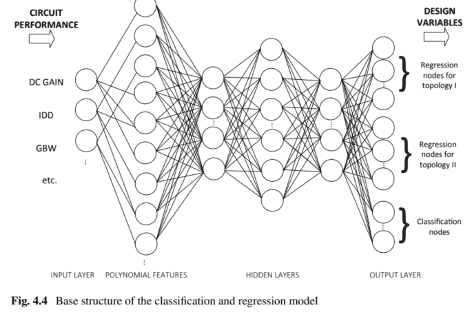
The ANN architecture considered in this section is similar to the one used for the regression-only model, but now there is an increased number of output nodes, as shown in Fig. 4.4. The input features are now not only restricted to one class of circuits, but to three. The features still correspond to the same four performance measures used in the regression-only model. The output layer is now not only comprised of a series of nodes that represent the circuit’s sizes, but also an additional node for each class of circuits present in the dataset. The loss function used in the training of the networks will also be different, now taking into account both errors from the regression and the classification tasks. The weights assigned to each error measures are malleable, but weights of $70 \%$ and $30 \%$, respectively, were used as a starting point.

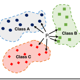
For this case study, three classes of circuits were considered. The output nodes responsible for classification assign a probability to the predicted class. Data preparation for this model involved the same steps of normalization and data augmentation through polynomial features as the ones from the regression-only model. The guidelines to select the hyper-parameters for the ANN classification and regression model architecture were as follows:

1. The number of input nodes and the number of hidden layers are the same as the regression-only model architecture. The number of nodes in the output layer increases in relation to the previous model, which are now 30 . This reflects the fact that the network is now processing different circuit performances and target circuit measures: 12 nodes for the VCOTA topology and 15 nodes for the twostage Miller amplifier topology, and 3 additional nodes that encode the circuit class.
2. The activation function used in all nodes (except in the output layer’ nodes) is ReLU.
3. Adam was the chosen optimizer, with learning rate $=0.001$.
4. Overfitting was addressed using $L_{2}$ weight regularization, as shown in Fig. $4.5$,after the model showed to have a good performance.
5. Initial random weights of the network layers were initialized by means of a normal distribution.
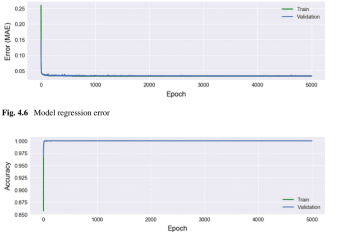
6. Model performance was measured through a custom loss function (see Eq. 4.8) that takes into account the error measurements from the classification nodes and from the regression nodes. Different percentages are assigned to each type of error, $30 \%$ and $70 \%$, respectively. Individual metrics were also used to prove the effectiveness of each task in the network. Regression error is calculated though a MSE function, while classification error is calculated through a sparse softmax cross-entropy (SSCE) function.
7. 5000 was the number of epochs chosen for initial testing. After having trained the first model, subsequent ANNs were trained with fewer epochs (500), using network weights from the ANN trained for 5000 epochs.
8. A variable number was chosen for batch size, between 256 and 512, depending on the number of epochs.
9. Finally, gridsearch is once again done over the hyper-parameters (number of layer, number of nodes per layer, non-ideality, and regularization factor) to finetune the model.

The hyper-parameters chosen for this architecture are summarized in Table 4.2.

电子工程代写|电路设计作业代写Intro to circuit design代考|Training

The loss function, $L_{2}$, of the model that is optimized during training is a weighted sum of two distinct losses-one from the regression task and the other from the classification task. Since this model’s input features are not restricted to only one class of circuit performances, the regression loss will itself be a sum of the training errors from each circuit included in the dataset. Each individual regression loss is determined using MSE, like the previous model, while the classification error is measured through a SSCE function. This function measures the probability error in discrete classification tasks in which the classes are mutually exclusive (each entry is in exactly one class).

The loss function, $L_{\text {class }}$, that is optimized for the classification task is obtained by computing the negative logarithm of the probability of the true class, i.e., the class with highest probability as predicted by the ANN:
$$
L_{\text {class }}=-\log \left(p\left(Y_{\text {class }}\right)\right)
$$
The loss function, $L_{\text {reg, }}$, that is optimized for the regression task is the MSE of predicted outputs $Y^{\prime}$ with respect to the true $Y$ plus the $L_{2}$ norm of the model’s weights, $W$, times the regularization factor $\lambda$ :
$$
L_{\mathrm{reg}}=\frac{1}{M} \sum_{j=1}^{M}\left(\left(Y_{\langle j\rangle}^{\prime}-Y_{\langle j\rangle}\right)^{T}\left(Y_{\langle j\rangle}^{\prime}-Y_{\langle j\rangle}\right)\right)+\lambda|W|^{2}
$$

电路设计作业代写

电子工程代写|电路设计作业代写INTRO TO CIRCUIT DESIGN代考|CLASSIFICATION AND REGRESSION MODEL

本节考虑的 ANN 架构类似于仅用于回归模型的架构，但现在输出节点的数量有所增加，如图 4.4 所示。输入特征现在不仅限于一类电路，而是三类。这些特征仍然对应于仅回归模型中使用的相同的四个性能度量。输出层现在不仅由代表电路大小的一系列节点组成，而且还包含数据集中存在的每一类电路的附加节点。网络训练中使用的损失函数也将有所不同，现在考虑到回归和分类任务的误差。分配给每个误差度量的权重是可塑的，但权重70%和30%，分别作为起点。

在本案例研究中，考虑了三类电路。负责分类的输出节点将概率分配给预测的类。该模型的数据准备涉及通过多项式特征进行归一化和数据增强的步骤，这些步骤与仅回归模型中的步骤相同。为 ANN 分类和回归模型架构选择超参数的指南如下：

1. 输入节点的数量和隐藏层的数量与仅回归模型架构相同。输出层中的节点数量相对于之前的模型增加了，现在是 30 。这反映了网络现在正在处理不同的电路性能和目标电路测量的事实：VCOTA 拓扑的 12 个节点和两级米勒放大器拓扑的 15 个节点，以及对电路类别进行编码的 3 个附加节点。
2. 所有节点使用的激活函数和XC和p吨一世n吨H和这在吨p在吨l一种是和r′n这d和s是Relu。
3. Adam 是选择的优化器，具有学习率=0.001.
4. 过度拟合是使用解决的大号2权重正则化，如图所示。4.5, 后模型表现出良好的表现。
5. 网络层的初始随机权重通过正态分布进行初始化。
6. 通过自定义损失函数测量模型性能s和和和q.4.8这考虑了来自分类节点和回归节点的误差测量。为每种类型的错误分配不同的百分比，30%和70%， 分别。个人指标也被用来证明网络中每个任务的有效性。回归误差通过 MSE 函数计算，而分类误差通过稀疏 softmax 交叉熵计算小号小号C和功能。
7. 5000 是为初始测试选择的 epoch 数。在训练了第一个模型之后，后续的 ANN 训练的 epoch 更少500，使用来自 ANN 训练了 5000 个 epoch 的网络权重。
8. 根据 epoch 的数量，为批量大小选择了一个可变数字，介于 256 和 512 之间。
9. 最后，再次对超参数进行网格搜索n在米b和r这Fl一种是和r,n在米b和r这Fn这d和sp和rl一种是和r,n这n−一世d和一种l一世吨是,一种ndr和G在l一种r一世和一种吨一世这nF一种C吨这r微调模型。

表 4.2 总结了为该架构选择的超参数。

电子工程代写|电路设计作业代写INTRO TO CIRCUIT DESIGN代考|TRAINING

损失函数，大号2，在训练期间优化的模型是两个不同损失的加权和 – 一个来自回归任务，另一个来自分类任务。由于该模型的输入特征不仅限于一类电路性能，因此回归损失本身将是数据集中每个电路的训练误差之和。与之前的模型一样，每个单独的回归损失都是使用 MSE 确定的，而分类误差是通过 SSCE 函数测量的。此函数测量类别互斥的离散分类任务中的概率误差和一种CH和n吨r是一世s一世n和X一种C吨l是这n和Cl一种ss.

损失函数，大号班级 ，通过计算真实类的概率的负对数来获得针对分类任务的优化，即由人工神经网络预测的具有最高概率的类：
$$
L_{\text {class }}=-\log \left(p\left(Y_{\text {class }}\right)\right)
$$
损失函数，大号注册， ，为回归任务优化的是预测输出的 MSE是′关于真实的是加上大号2模型权重的范数，在, 乘以正则化因子λ :
$$
L_{\mathrm{reg}}=\frac{1}{M} \sum_{j=1}^{M}\left(\left(Y_{\langle j\rangle}^{\prime}-Y_{\langle j\rangle}\right)^{T}\left(Y_{\langle j\rangle}^{\prime}-Y_{\langle j\rangle}\right)\right)+\lambda|W|^{2}
$$

电子工程代写|电路设计作业代写Intro to circuit design代考 请认准UprivateTA™. UprivateTA™为您的留学生涯保驾护航。

电磁学代考

物理代考服务：
物理Physics考试代考、留学生物理online exam代考、电磁学代考、热力学代考、相对论代考、电动力学代考、电磁学代考、分析力学代考、澳洲物理代考、北美物理考试代考、美国留学生物理final exam代考、加拿大物理midterm代考、澳洲物理online exam代考、英国物理online quiz代考等。

光学代考

光学（Optics），是物理学的分支，主要是研究光的现象、性质与应用，包括光与物质之间的相互作用、光学仪器的制作。光学通常研究红外线、紫外线及可见光的物理行为。因为光是电磁波，其它形式的电磁辐射，例如X射线、微波、电磁辐射及无线电波等等也具有类似光的特性。

大多数常见的光学现象都可以用经典电动力学理论来说明。但是，通常这全套理论很难实际应用，必需先假定简单模型。几何光学的模型最为容易使用。

相对论代考

上至高压线，下至发电机，只要用到电的地方就有相对论效应存在！相对论是关于时空和引力的理论，主要由爱因斯坦创立，相对论的提出给物理学带来了革命性的变化，被誉为现代物理性最伟大的基础理论。

流体力学代考

流体力学是力学的一个分支。 主要研究在各种力的作用下流体本身的状态，以及流体和固体壁面、流体和流体之间、流体与其他运动形态之间的相互作用的力学分支。

随机过程代写

随机过程，是依赖于参数的一组随机变量的全体，参数通常是时间。 随机变量是随机现象的数量表现，其取值随着偶然因素的影响而改变。 例如，某商店在从时间t0到时间tK这段时间内接待顾客的人数，就是依赖于时间t的一组随机变量，即随机过程

Matlab代写

MATLAB 是一种用于技术计算的高性能语言。它将计算、可视化和编程集成在一个易于使用的环境中，其中问题和解决方案以熟悉的数学符号表示。典型用途包括：数学和计算算法开发建模、仿真和原型制作数据分析、探索和可视化科学和工程图形应用程序开发，包括图形用户界面构建MATLAB 是一个交互式系统，其基本数据元素是一个不需要维度的数组。这使您可以解决许多技术计算问题，尤其是那些具有矩阵和向量公式的问题，而只需用 C 或 Fortran 等标量非交互式语言编写程序所需的时间的一小部分。MATLAB 名称代表矩阵实验室。MATLAB 最初的编写目的是提供对由 LINPACK 和 EISPACK 项目开发的矩阵软件的轻松访问，这两个项目共同代表了矩阵计算软件的最新技术。MATLAB 经过多年的发展，得到了许多用户的投入。在大学环境中，它是数学、工程和科学入门和高级课程的标准教学工具。在工业领域，MATLAB 是高效研究、开发和分析的首选工具。MATLAB 具有一系列称为工具箱的特定于应用程序的解决方案。对于大多数 MATLAB 用户来说非常重要，工具箱允许您学习和应用专业技术。工具箱是 MATLAB 函数（M 文件）的综合集合，可扩展 MATLAB 环境以解决特定类别的问题。可用工具箱的领域包括信号处理、控制系统、神经网络、模糊逻辑、小波、仿真等。