数学代写|Least-norm problems 凸优化代考
凸优化代写
$6.2$ Least-norm problems
The basic least-norm problem has the form
$$
\begin{array}{ll}
\text { minimize } & |x| \
\text { subject to } & A x=b
\end{array}
$$
where the data are $A \in \mathbf{R}^{m \times n}$ and $b \in \mathbf{R}^{m}$, the variable is $x \in \mathbf{R}^{n}$, and $|\cdot|$ is norm on $\mathbf{R}^{n}$. A solution of the problem, which always exists if the linear equation $A x=b$ have a solution, is called a least-norm solution of $A x=b .$ The least-nor problem is, of course, a convex optimization problem.
We can assume without loss of generality that the rows of $A$ are independent, $m \leq n .$ When $m=n$, the only feasible point is $x=A^{-1} b ;$ the least-norm problen is interesting only when $m<n$, i.e., when the equation $A x=b$ is underdetermined
$\mathrm{~ R e f o r m u l a t i o n ~ a s ~ n o r m ~ a p r o t e r}$
303
Reformulation as norm approximation problem
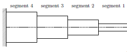
The least-norm problem $(6.5)$ can be formulated as a norm approximation problem by eliminating the equality constraint. Let $x_{0}$ be any solution of $A x=b$, and let $Z \in \mathbf{R}^{n \times k}$ be a matrix whose columns are a basis for the nullspace of $A$. The general solution of $A x=b$ can then be expres least-norm problem $(6.5)$ can be expressed as minimize $\left|x_{0}+Z u\right|$, with variable $u \in \mathbf{R}^{k}$, which is a norm approximation problem. In particular, ur analysis and discussion of norm approximation problems applies to least-norm roblems as well (when interpreted correctly). Control or design interpretation optimal control. The $n$ variables $x_{1}, \ldots, x_{n}$ are design variables whose values are to be determined. In a control setting, the variables $x_{1}, \ldots, x_{n}$ represent inputs, whose values we are to choose. The vector $y=A x$ gives $m$ attributes or results of the design $x$, which we assume to be linear functions of the design variables $x$. The $m<n$ equations $A x=b$ represent $m$ specifications or requirements on the design. Since $m<n$, the design is underspecified; there are $n-m$ degrees of freedom in the design (assuming $A$ is rank $m)$. Among all the designs that satisfy the specifications, the least-norm problem chooses the smallest design, as measured by the norm $|\cdot| .$ This can be thought of as the most efficient design, in the sense that it achieves the specifications $A x=b$, with the smallest possible $x$.
Estimation interpretation
We assume that $x$ is a vector of parameters to be estimated. We have $m<n$ perfect (noise free) linear measurements, given by $A x=b$. Since we have fewer measurements than parameters to estimate, our measurements do not completely determine $x .$ Any parameter vector $x$ that satisfies $A x=b$ is consistent with our measurements.
To make a good guess about what $x$ is, without taking further measurements, we must use prior information. Suppose our prior information, or assumption, is that $x$ is more likely to be small (as measured by $|\cdot|$ ) than large. The least-norm problem chooses as our estimate of the parameter vector $x$ the one that is smallest (hence, most plausible) among all parameter vectors that are consistent with the measurements $A x=b$. (For a statistical interpretation of the least-norm problem, see page 359.)
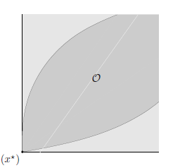
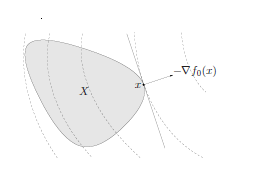
Geometric interpretation
We can also give a simple geometric interpretation of the least-norm problem $(6.5)$. The feasible set ${x \mid A x=b}$ is affine, and the objective is the distance (measured by the norm $|\cdot|$ ) between $x$ and the point 0 . The least-norm problem finds the

凸优化代考
$6.2$ 最小范数问题
基本最小范数问题的形式为
$$
\开始{数组}{ll}
\text { 最小化 } & |x| \
\text { 服从 } & A x=b
\结束{数组}
$$
其中数据为 $A \in \mathbf{R}^{m \times n}$ 和 $b \in \mathbf{R}^{m}$,变量为 $x \in \mathbf{R}^ {n}$,$|\cdot|$ 是 $\mathbf{R}^{n}$ 上的范数。如果线性方程 $A x=b$ 有解,则该问题的解称为 $A x=b 的最小范数解。当然,最小或非问题是凸的优化问题。
我们可以不失一般性假设 $A$ 的行是独立的,$m \leq n .$ 当 $m=n$ 时,唯一可行的点是 $x=A^{-1} b ;$ 最少-norm problen 仅在 $m<n$ 时才有意义,即当方程 $A x=b$ 未确定时
$\mathrm{~ R e f o r m u l a t i o n ~ a s ~ n o r m ~ a p r o t e r}$
303
重新表述为范数逼近问题
通过消除等式约束,最小范数问题$(6.5)$ 可以表述为范数逼近问题。令 $x_{0}$ 是 $A x=b$ 的任意解,令 $Z \in \mathbf{R}^{n \times k}$ 是一个矩阵,其列是 $ 的零空间的基础澳元。 $A x=b$ 的通解可以表示为最小范数问题 $(6.5)$ 可以表示为最小化 $\left|x_{0}+Z u\right|$,变量 $u \in \mathbf{R}^{k}$,这是一个范数逼近问题。特别是,您对范数逼近问题的分析和讨论也适用于最小范数问题(如果解释正确)。控制或设计解释最优控制。 $n$ 变量 $x_{1}、\ldots、x_{n}$ 是要确定其值的设计变量。在控制设置中,变量 $x_{1}、\ldots、x_{n}$ 代表输入,我们将选择其值。向量 $y=A x$ 给出了设计 $x$ 的 $m$ 属性或结果,我们假设它们是设计变量 $x$ 的线性函数。 $m<n$ 方程 $A x=b$ 代表 $m$ 规范或设计要求。由于 $m<n$,设计未指定;设计中有 $n-m$ 个自由度(假设 $A$ 是秩 $m)$。在所有满足规范的设计中,最小范数问题选择最小的设计,以范数 $|\cdot| 衡量。 .$ 这可以被认为是最有效的设计,因为它实现了规范 $A x=b$,并且具有尽可能小的 $x$。
估计解释
我们假设 $x$ 是要估计的参数向量。我们有 $m<n$ 完美(无噪声)线性测量,由 $A x=b$ 给出。由于我们的测量值少于要估计的参数,因此我们的测量值并不能完全确定 $x。$ 任何满足 $A x=b$ 的参数向量 $x$ 都与我们的测量值一致。
为了很好地猜测 $x$ 是什么,在不进行进一步测量的情况下,我们必须使用先验信息。假设我们的先验信息或假设是 $x$ 更可能是小(由 $|\cdot|$ 衡量)而不是大。最小范数问题选择与测量值 $A x=b$ 一致的所有参数向量中最小的(因此,最合理的)作为我们对参数向量 $x$ 的估计。 (有关最小范数问题的统计解释,请参见第 359 页。)
几何解释
我们还可以对最小范数问题 $(6.5)$ 给出一个简单的几何解释。可行集 ${x \mid A x=b}$ 是仿射的,目标是 $x$ 和点 0 之间的距离(由范数 $|\cdot|$ 测量)。最小范数问题找到

数学代写| Chebyshev polynomials 数值分析代考 请认准UprivateTA™. UprivateTA™为您的留学生涯保驾护航。
时间序列分析代写
统计作业代写
随机过程代写
随机过程,是依赖于参数的一组随机变量的全体,参数通常是时间。 随机变量是随机现象的数量表现,其取值随着偶然因素的影响而改变。 例如,某商店在从时间t0到时间tK这段时间内接待顾客的人数,就是依赖于时间t的一组随机变量,即随机过程