数学代写|Linear optimization problems 凸优化代考
凸优化代写
Least-squares and regression
The problem of minimizing the convex quadratic function
$$
|A x-b|_{2}^{2}=x^{T} A^{T} A x-2 b^{T} A x+b^{T} b
$$
is an (unconstrained) QP. It arises in many fields and has many names, e.g., regression analysis or least-squares approximation. This problem is simple enough to have the well known analytical solution $x=A^{\dagger} b$, where $A^{\dagger}$ is the pseudo-inverse of $A$ (see $\$ \mathrm{~A} .5 .4$ ).
When linear inequality constraints are added, the problem is called constrained regression or constrained least-squares, and there is no longer a simple analytical solution. As an example we can consider regression with lower and upper bounds on the variables, i.e.,
$$
\begin{array}{ll}
\text { minimize } & |A x-b|_{2}^{2} \
\text { subject to } & l_{i} \leq x_{i} \leq u_{i}, \quad i=1, \ldots, n
\end{array}
$$
4 Convex optimization problems
154
which is a QP. (We will study least-squares and regression problems in far more depth in chapters 6 and 7 .)
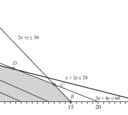
Distance between polyhedra
The (Euclidean) distance between the polyhedra $\mathcal{P}{1}=\left{x \mid A{1} x \preceq b_{1}\right}$ and $\mathcal{P}{2}=$ $\left{x \mid A{2} x \preceq b_{2}\right}$ in $\mathbf{R}^{n}$ is defined as
$$
\operatorname{dist}\left(\mathcal{P}{1}, \mathcal{P}{2}\right)=\inf \left{\left|x_{1}-x_{2}\right|_{2} \mid x_{1} \in \mathcal{P}{1}, x{2} \in \mathcal{P}{2}\right} $$ If the polyhedra intersect, the distance is zero. To find the distance between $\mathcal{P}{1}$ and $\mathcal{P}{2}$, we can solve the $Q P$ $$ \begin{array}{ll} \text { minimize } & \left|x{1}-x_{2}\right|_{2}^{2} \
\text { subject to } & A_{1} x_{1} \preceq b_{1}, \quad A_{2} x_{2} \preceq b_{2}
\end{array}
$$
with variables $x_{1}, x_{2} \in \mathbf{R}^{n}$. This problem is infeasible if and only if one of the polyhedra is empty. The optimal value is zero if and only if the polyhedra intersect, in which case the optimal $x_{1}$ and $x_{2}$ are equal (and is a point in the intersection $\mathcal{P}{1} \cap \mathcal{P}{2}$ ). Otherwise the optimal $x_{1}$ and $x_{2}$ are the points in $\mathcal{P}{1}$ and $\mathcal{P}{2}$, respectively, that are closest to each other. (We will study geometric problems involving distance in more detail in chapter 8.)
Bounding variance
We consider again the Chebyshev inequalities example (page 150 ), where the variable is an unknown probability distribution given by $p \in \mathbf{R}^{n}$, about which we have some prior information. The variance of a random variable $f(x)$ is given by
$$
\mathbf{E} f^{2}-(\mathbf{E} f)^{2}=\sum_{i=1}^{n} f_{i}^{2} p_{i}-\left(\sum_{i=1}^{n} f_{i} p_{i}\right)^{2}
$$
(where $f_{1}=f\left(u_{i}\right)$ ), which is a concave quadratic function of $p$.
It follows that we can maximize the variance of $f(x)$, subject to the given prior information, by solving the $Q P$
$$
\begin{array}{ll}
\text { maximize } & \sum_{i=1}^{n} f_{i}^{2} p_{i}-\left(\sum_{i-1}^{n} f_{i} p_{i}\right)^{2} \
\text { subject to } & p \succeq 0, \quad 1^{T} p=1 \
& \alpha_{i} \leq a_{i}^{T} p \leq \beta_{i}, \quad i=1, \ldots, m .
\end{array}
$$
The optimal value gives the maximum possible variance of $f(x)$, over all distributions that are consistent with the prior information; the optimal $p$ gives a distribution that achieves this maximum variance.
Linear program with random cost
We consider an LP,
$$
\begin{array}{ll}
\text { minimize } & c^{T} x \
\text { subject to } & G x \preceq h \
& A x=b
\end{array}
$$
155
4.4 Quadratic optimization problems
with variable $x \in \mathbf{R}^{n}$. We suppose that the cost function (vector) $c \in \mathbf{R}^{n}$ is random, with mean value $\bar{c}$ and covariance $\mathbf{E}(c-\bar{c})(c-\bar{c})^{T}=\Sigma$. (We assume for simplicity that the other problem parameters are deterministic.) For a given $x \in \mathbf{R}^{n}$, the cost $c^{T} x$ is a (scalar) random variable with mean $\mathbf{E} c^{T} x=\bar{c}^{T} x$ and variance
$$
\operatorname{var}\left(c^{T} x\right)=\mathbf{E}\left(c^{T} x-\mathbf{E} c^{T} x\right)^{2}=x^{T} \Sigma x
$$
In general there is a trade-off between small expected cost and small cost variance. One way to take variance into account is to minimize a linear combination of the expected value and the variance of the cost, i.e.,
$$
\mathbf{E} c^{T} x+\gamma \operatorname{var}\left(c^{T} x\right)
$$
which is called the risk-sensitive cost. The parameter $\gamma \geq 0$ is called the riskaversion parameter, since it sets the relative values of cost variance and expected value. (For $\gamma>0$, we are willing to trade off an increase in expected cost for $\mathrm{a}$ sufficiently large decrease in cost variance).
To minimize the risk-sensitive cost we solve the $Q P$
Markowitz portfolio optimization
We consider a classical portfolio problem with $n$ assets or stocks held over a period of time. We let $x_{i}$ denote the amount of asset $i$ held throughout the period, with $x_{i}$ in dollars, at the price at the beginning of the period. A normal long position in asset $i$ corresponds to $x_{0}>0$; a short position in asset $i$ (i.e., the obligation to buy the asset at the end of the period) corresponds to $x_{1}<0$. We let $p_{i}$ denote the relative price change of asset $i$ over the period, i.e., its change in price over the period divided by its price at the beginning of the period. The overall return on the portfolio is $r=p^{T} x$ (given in dollars). The optimization variable is the portfolio vector $x \in \mathbf{R}^{n}$.
A wide variety of constraints on the portfolio can be considered. The simplest set of constraints is that $x_{1} \geq 0$ (ie., no short positions) and $1^{T} x=B$ (ie., the total budget to be invested is $B$, which is often taken to be one).
We trake a stochastic model for price changes: $p \in \mathbf{R}^{n}$ is a random vector, with known mean $\bar{p}$ and covariance $\Sigma$. Therefore with portfolio $x \in \mathbf{R}^{\mathrm{n}}$, the return $r$ is a (scalar) random variable with mean $\bar{p}^{T} x$ and variance $x^{T} \Sigma x$. The choice of portfolio $x$ involves a trade-off between the mean of the return, and its variance.
The classical portfolio optimization problem, introduced by Markowitz, is the $Q P$
$$
\begin{array}{ll}
\text { minimize } & x^{T} \Sigma x \
\text { subject to } & \bar{p}^{T} x \geq r_{\min } \
& 1^{T} x=1, \quad x \geq 0
\end{array}
$$
the portfolio) subject to where $r$, the portfolio, is the variable. Here we find the portfolio that minimizes
4 Convex optimization problems
achieving a minimum acceptable mean return $r_{\text {min }}$, and satisfying the portfolio budget and no-shorting constraints.
Many extensions are possible. One standard extension, for example, is to allow short positions, ie., $x_{1}<0$. To do this we introduce variables $x_{\text {lang }}$ and $x_{\text {short }}$, with
$x_{\text {long }} \succeq 0, \quad x_{\text {short }} \succeq 0, \quad x=x_{\text {long }}-x_{\text {shart }}, \quad 1^{T} x_{\text {short }} \leq \eta 1^{T} x_{\text {long }} .$
The last constraint limits the total short position at the beginning of the period to some fraction $\eta$ of the total long position at the beginning of the period.
As another extension we can include linear transaction costs in the portfolio optimization problem. Starting from a given initial portfolio $x_{\text {init }}$ we buy and sell assets to achieve the portfolio $x$, which we then hold over the period as described shove. We are charged a transaction fee for buying and selling assets, which is proportional to the amount bought or sold. To handle this, we introduce variables $u_{\text {buy }}$ and $u_{\text {soll, }}$, which determine the amount of each asset we buy and sell before the holding period. We have the constraints
minimize $x^{T} \Sigma x$
subject to $\bar{p}^{T} x \geq r_{\text {min }}$
$$
1^{T} x=1, \quad x \geq 0
$$
where $x$, the portfolio, is the variable. Here we find the portfolio that minimizes the return variance (which is associated with the risk of the portfolio) subject to
凸优化代考
最小二乘和回归
凸二次函数最小化问题
$$
|A x-b|_{2}^{2}=x^{T} A^{T} A x-2 b^{T} A x+b^{T} b
$$
是一个(无约束的)QP。它出现在许多领域并有许多名称,例如回归分析或最小二乘近似。这个问题很简单,有众所周知的解析解 $x=A^{\dagger} b$,其中 $A^{\dagger}$ 是 $A$ 的伪逆(参见 $\$ \mathrm{ ~A} .5 .4$ )。
当加入线性不等式约束时,该问题称为约束回归或约束最小二乘,不再有简单的解析解。作为一个例子,我们可以考虑对变量有下限和上限的回归,即
$$
\开始{数组}{ll}
\text { 最小化 } & |A x-b|_{2}^{2} \
\text { 服从 } & l_{i} \leq x_{i} \leq u_{i}, \quad i=1, \ldots, n
\结束{数组}
$$
4 凸优化问题
154
这是一个QP。 (我们将在第 6 章和第 7 章更深入地研究最小二乘和回归问题。)
多面体之间的距离
多面体 $\mathcal{P}{1}=\left{x \mid A{1} x \preceq b_{1}\right}$ 和 $\mathcal{P}_ 之间的(欧几里得)距离$\mathbf{R}^{n}$ 中的 {2}=$ $\left{x \mid A_{2} x \preceq b_{2}\right}$ 定义为
$$
\operatorname{dist}\left(\mathcal{P}{1}, \mathcal{P}{2}\right)=\inf \left{\left|x_{1}-x_{2} \right|_{2} \mid x_{1} \in \mathcal{P}{1}, x{2} \in \mathcal{P}{2}\right} $$ 如果多面体相交,则距离为零。 要找到 $\mathcal{P}{1}$ 和 $\mathcal{P}{2}$ 之间的距离,我们可以求解 $Q P$ $$ \开始{数组}{ll} \text { 最小化 } & \left|x{1}-x_{2}\right|_{2}^{2} \
\text { 服从 } & A_{1} x_{1} \preceq b_{1}, \quad A_{2} x_{2} \preceq b_{2}
\结束{数组}
$$
带有变量 $x_{1}, x_{2} \in \mathbf{R}^{n}$。当且仅当多面体之一为空时,此问题是不可行的。当且仅当多面体相交时,最优值为零,在这种情况下,最优 $x_{1}$ 和 $x_{2}$ 相等(并且是交叉点 $\mathcal{P}{1 } \cap \mathcal{P}{2}$)。否则,最优 $x_{1}$ 和 $x_{2}$ 分别是 $\mathcal{P}{1}$ 和 $\mathcal{P}{2}$ 中最接近于彼此。 (我们将在第 8 章更详细地研究涉及距离的几何问题。)
边界方差
我们再次考虑 Chebyshev 不等式示例(第 150 页),其中变量是由 $p \in \mathbf{R}^{n}$ 给出的未知概率分布,我们有一些先验信息。随机变量 $f(x)$ 的方差由下式给出
$$
\mathbf{E} f^{2}-(\mathbf{E} f)^{2}=\sum_{i=1}^{n} f_{i}^{2} p_{i}-\left (\sum_{i=1}^{n} f_{i} p_{i}\right)^{2}
$$
(其中 $f_{1}=f\left(u_{i}\right)$ ),这是 $p$ 的凹二次函数。
因此,在给定先验信息的情况下,我们可以通过求解 $Q P$ 来最大化 $f(x)$ 的方差
$$
\开始{数组}{ll}
\text { 最大化 } & \sum_{i=1}^{n} f_{i}^{2} p_{i}-\left(\sum_{i-1}^{n} f_{i} p_{ i}\right)^{2} \
\text { 服从 } & p \succeq 0, \quad 1^{T} p=1 \
& \alpha_{i} \leq a_{i}^{T} p \leq \beta_{i}, \quad i=1, \ldots, m 。
\结束{数组}
$$
在与先验信息一致的所有分布上,最优值给出了 $f(x)$ 的最大可能方差;最优 $p$ 给出了一个达到这个最大方差的分布。
具有随机成本的线性规划
我们考虑一个LP,
$$
\开始{数组}{ll}
\text { 最小化 } & c^{T} x \
\text { 服从 } & G x \preceq h \
& A x=b
\结束{数组}
$$
155
4.4 二次优化问题
带有变量 $x \in \mathbf{R}^{n}$。我们假设成本函数(向量)$c \in \mathbf{R}^{n}$ 是随机的,具有平均值 $\bar{c}$ 和协方差 $\mathbf{E}(c-\bar{ c})(c-\bar{c})^{T}=\Sigma$。 (为简单起见,我们假设其他问题参数是确定性的。)对于给定的 $x \in \mathbf{R}^{n}$,成本 $c^{T} x$ 是一个(标量)随机变量均值 $\mathbf{E} c^{T} x=\bar{c}^{T} x$ 和方差
$$
\operatorname{var}\left(c^{T} x\right)=\mathbf{E}\left(c^{T} x-\mathbf{E} c^{T} x\right)^{2 }=x^{T} \Sigma x
$$
一般来说,在较小的预期成本和较小的成本差异之间存在权衡。考虑方差的一种方法是最小化期望值和成本方差的线性组合,即
$$
\mathbf{E} c^{T} x+\gamma \operatorname{var}\left(c^{T} x\right)
$$
这称为风险敏感成本。参数$\gamma\geq 0$ 被称为风险规避参数,因为它设置了成本方差和期望值的相对值。 (对于 $\gamma>0$,我们愿意用预期成本的增加来换取 $\mathrm{a}$ 足够大的成本方差降低)。
为了最小化风险敏感成本,我们求解 $Q P$
马科维茨投资组合优化
我们考虑一个经典的投资组合问题,在一段时间内持有 $n$ 资产或股票。我们让 $x_{i}$ 表示在整个期间持有的资产 $i$ 的数量,$x_{i}$ 以美元为单位,在 t

数学代写| Chebyshev polynomials 数值分析代考 请认准UprivateTA™. UprivateTA™为您的留学生涯保驾护航。
时间序列分析代写
统计作业代写
随机过程代写
随机过程,是依赖于参数的一组随机变量的全体,参数通常是时间。 随机变量是随机现象的数量表现,其取值随着偶然因素的影响而改变。 例如,某商店在从时间t0到时间tK这段时间内接待顾客的人数,就是依赖于时间t的一组随机变量,即随机过程