数学代写|Regularized approximation 凸优化代考
凸优化代写
In the basic form of regularized approximation, the goal is to find a vector $x$ that is small (if possible), and also makes the residual $A x-b$ small. This is naturally described as a (convex) vector optimization problem with two objectives, $|A x-b|$ and $|x|$ :
$\operatorname{minimize}\left(\right.$ w.r.t. $\left.\mathbf{R}_{+}^{2}\right) \quad(|A x-b|,|x|)$.
The two norms can be different: the first, used to measure the size of the residual, is on $\mathbf{R}^{m}$; the second, used to measure the size of $x$, is on $\mathbf{R}^{n}$.
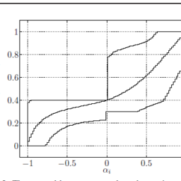
The optimal trade-off between the two objectives can be found using several methods. The optimal trade-off curve of $|A x-b|$ versus $|x|$, which shows how large one of the objectives must be made to have the other one small, can then be plotted. One endpoint of the optimal trade-off curve between $|A x-b|$ and $|x|$ is easy to describe. The minimum value of $|x|$ is zero, and is achieved only when $x=0$. For this value of $x$, the residual norm has the value $|b|$.
The other endpoint of the trade-off curve is more complicated to describe. Let $C$ denote the set of minimizers of $|A x-b|$ (with no constraint on $|x|)$. Then any minimum norm point in $C$ is Pareto optimal, corresponding to the other endpoint of the trade-off curve. In other words, Pareto optimal points at this endpoint are given by minimum norm minimizers of $|A x-b|$. If both norms are Euclidean, this Pareto optimal point is unique, and given by $x=A^{\dagger} b$, where $A^{\dagger}$ is the pseudoinverse of $A$. (See $\S 4.7 .6$, page 184, and §A.5.4.)
(See ).7.6, page 184, and §A.5.4.) 306 Approximation and fitting
6.3.2 Regularization
Regularization is a common scalarization method used to solve the bi-criterion problem (6.7). One form of regularization is to minimize the weighted sum of the objectives:
where $\gamma>0$ is a problem parameter. As $\gamma$ varies over $(0,$, traces out the optimal trade-off curve. Another common method of regularization, especially is used, is to minimize the weighted sum of squared nor for a variety of values of $\delta>0$. These regularized approximation problems each solve of making both $|A x-b|$ and $|x|$ small, by adding associated with the norm of $x$. Interpretations
Regularization is used in several contexts. In an estimation setting, the extra term penalizing large $|x|$ can be interpreted as our prior knowledge that $|x|$ is not too large. In an optimal design setting, the extra term adds the cost of using large values of the design variables to the cost of missing the target specifications.
The constraint that $|x|$ be small can also reflect a modeling issue. It might be, for example, that $y=A x$ is only a good approximation of the true relationship $y=f(x)$ between $x$ and $y .$ In order to have $f(x) \approx b$, we want $A x \approx b$, and also $y=f(x)$ between $x$ and $y .$ In order to have $f(x)$ Weed $x$ small in order to ensure that $f(x) \approx A x . } \{\text { We in } 86.4 .1 \text { and } 86.4 .2 \text { that regularization can be used to take into }} \end{array}$ account variation in the matrix $A$. Roughly speaking, a large $x$ is one for which variation in $A$ causes large variation in $A x$, and hence should be avoided.
Regularization is also used when the matrix $A$ is square, and the goal is to solve the linear equations $A x=b .$ In cases where $A$ is poorly conditioned, or even singular, regularization gives a compromise between solving the equations (i.e., making $|A x-b|$ zero) and keeping $x$ of reasonable size.
Regularization comes up in a statistical setting; see $\$ 7.1 .2 .$
Tikhonov regularization
The most common form of regularization is based on $(6.9)$, with Euclidean norms, which results in a (convex) quadratic optimization problem:
minimize $\quad|A x-b|_{2}^{2}+\delta|x|_{2}^{2}=x^{T}\left(A^{T} A+\delta I\right) x-2 b^{T} A x+b^{T} b .$ This Tikhonov regularization problem has the analytical solution
$\begin{aligned} x &=\left(A^{T} A+\delta I\right)^{-1} A^{T} b . \ \text { Since } A^{T} A+\delta I \succ 0 \text { for any } \delta>0, \text { the Tikhonov regularized least-squares solution } \end{aligned}$ requires no rank (or dimension) assumptions on the matrix $A$.
凸优化代考
在正则化近似的基本形式中,目标是找到一个小的向量$x$(如果可能的话),同时也使残差$A x-b$ 小。这自然被描述为具有两个目标的(凸)向量优化问题,$|A x-b|$ 和 $|x|$:
$\operatorname{最小化}\left(\right.$ wrt $\left.\mathbf{R}_{+}^{2}\right) \quad(|A xb|,|x|)美元。
这两个规范可以不同:第一个,用于衡量残差的大小,在 $\mathbf{R}^{m}$ 上;第二个,用于测量 $x$ 的大小,在 $\mathbf{R}^{n}$ 上。
可以使用多种方法找到两个目标之间的最佳权衡。然后可以绘制 $|A x-b|$ 与 $|x|$ 的最佳权衡曲线,该曲线显示必须使一个目标变得多大才能使另一个目标变小。 $|A x-b|$ 和 $|x|$ 之间的最优权衡曲线的一个端点很容易描述。 $|x|$ 的最小值为零,只有当$x=0$ 时才达到。对于这个 $x$ 的值,残差范数的值为 $|b|$。
权衡曲线的另一个端点更难以描述。令$C$ 表示$|A x-b|$ 的最小化集合(对$|x| 没有约束)$。那么 $C$ 中的任何最小范数点都是帕累托最优的,对应于权衡曲线的另一个端点。换句话说,该端点的帕累托最优点由 $|A x-b|$ 的最小范数最小化器给出。如果两个范数都是欧几里得,这个帕累托最优点是唯一的,并且由 $x=A^{\dagger} b$ 给出,其中 $A^{\dagger}$ 是 $A$ 的伪逆。 (参见 $\S 4.7 .6$,第 184 页和 §A.5.4。)
(见 ).7.6,第 184 页和 §A.5.4。) 306 近似和拟合
6.3.2 正则化
正则化是用于解决双准则问题 (6.7) 的常用标量化方法。正则化的一种形式是最小化目标的加权和:
其中 $\gamma>0$ 是一个问题参数。当$\gamma$ 在$(0,$ 上变化时,描绘出最优的权衡曲线。另一种常用的正则化方法,特别是使用的,是最小化加权平方和,也不是对于$\delta 的各种值>0$。这些正则化近似问题都通过与 $x$ 的范数相加来解决使 $|A xb|$ 和 $|x|$ 都变小的问题。
正则化在多种情况下使用。在估计设置中,惩罚大 $|x|$ 的额外项可以解释为我们的先验知识,即 $|x|$ 不是太大。在最佳设计设置中,额外项会将使用较大的设计变量值的成本添加到缺少目标规范的成本中。
$|x|$ 小的约束也可以反映建模问题。例如,$y=A x$ 可能只是 $x$ 和 $y 之间真实关系 $y=f(x)$ 的良好近似。约 b$,我们想要 $A x \approx b$,并且 $y=f(x)$ 在 $x$ 和 $y 之间。$ 为了使 $f(x)$ 杂草 $x$ 小以确保 $f(x) \approx A x 。 } \{\text { 我们在 } 86.4 .1 \text { 和 } 86.4 .2 \text { 可以使用正则化来考虑 }} \end{array}$ 考虑矩阵 $A$ 中的变化。粗略地说,较大的 $x$ 是 $A$ 的变化会导致 $A x$ 的较大变化,因此应该避免。
当矩阵 $A$ 是方阵时也使用正则化,目标是求解线性方程 $A x=b 。方程(即,使$|A xb|$ 为零)并保持$x$ 的大小合理。
正则化出现在统计环境中;见 $\$ 7.1 .2 .$
Tikhonov 正则化
最常见的正则化形式是基于$(6.9)$,使用欧几里得范数,这会导致(凸)二次优化问题:
最小化 $\quad|A xb|_{2}^{2}+\delta|x|_{2}^{2}=x^{T}\left(A^{T} A+\ delta I\right) x-2 b^{T} A x+b^{T} b .$ 这个Tikhonov正则化问题有解析解
$\begin{aligned} x &=\left(A^{T} A+\delta I\right)^{-1} A^{T} b 。 \ \text { 由于 } A^{T} A+\delta I \succ 0 \text { 对于任何 } \delta>0,\text { Tikhonov 正则化最小二乘解 } \end{aligned}$ 不需要秩(或维度)对矩阵 $A$ 的假设。

数学代写| Chebyshev polynomials 数值分析代考 请认准UprivateTA™. UprivateTA™为您的留学生涯保驾护航。
时间序列分析代写
统计作业代写
随机过程代写
随机过程,是依赖于参数的一组随机变量的全体,参数通常是时间。 随机变量是随机现象的数量表现,其取值随着偶然因素的影响而改变。 例如,某商店在从时间t0到时间tK这段时间内接待顾客的人数,就是依赖于时间t的一组随机变量,即随机过程