物理代写| Example Oblique Coordinate System on a Plane 相对论代考
物理代写
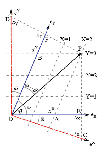
We will work out the formal algebra presented above for a two-dimensional toy case. We construct a coordinate system, where the constant ” $X$ ” and ” $Y$ ” lines are not orthogonal, but they are at an angle $\omega$, as shown in Fig. 3.2. This example has also been described in Narlikar $(2010)$, however here we give more details of the calculation.
Utilising the fact that vectors do not change under coordinate transformations, only their components do, we will compute all the quantities in an orthogonal Cartesian coordinate system. We use the lower case letters, $x$ and $y$, to represent this coordinate system. The $x$-axis is aligned with the $X=0$ line and the $y$-axis is orthogonal to the $x$-axis maintaining the right-hand rule at the common origin $\mathrm{O}$. In Fig. $3.2$, the $x$-axis (and the unit vector $\hat{\mathbf{i}}$ ) is coincident with the $\mathbf{e}_{X}$ direction and the $y$-axis (and the unit vector $\hat{\mathbf{j}}$ ) is coincident with the $\mathrm{e}^{Y}$ direction (reason for this overlap of axes will become clear in a moment).
An arbitrary point $\mathrm{P}$, which has the Cartesian coordinates $(x, y)$, will have coordinates $(X, Y)$ in the oblique coordinates following the relation
One can write the above coordinate transformation as
$$
\begin{aligned}
y &=Y \sin \omega \
x &=X+Y \cos \omega \
\Rightarrow \quad \mathbf{x} &:=\hat{\mathbf{i}} x+\hat{\mathbf{j}} y=\hat{\mathbf{i}}(X+Y \cos \omega)+\hat{\mathbf{j}} Y \sin \omega
\end{aligned}
$$
Thus we get the (covariant) basis for the contravariant components as
$$
\begin{aligned}
&\mathbf{e}{X}=\frac{\partial \mathbf{x}}{\partial X}=\hat{\mathbf{i}} \ &\mathbf{e}{Y}=\frac{\partial \mathbf{x}}{\partial Y}=\hat{\mathbf{i}} \cos \omega+\hat{\mathbf{j}} \sin \omega
\end{aligned}
$$
3.7 Example: Oblique Coordinate System on a Plane
53
The (contravariant) basis for the covariant components can be expressed as
$$
\begin{aligned}
\mathrm{e}^{X} &=\nabla X=\hat{\mathbf{i}}-\hat{\mathbf{j}} \cot \omega \
\mathrm{e}^{Y} &=\nabla Y=\hat{\mathbf{j}} / \sin \omega .
\end{aligned}
$$
Following the above expressions, the direction of the basis vectors have been marked in Fig. 3.2. Although the directions have been marked, the units along different axes are different, as reflected in the amplitude of the basis vectors. For example, unit of length along $\mathrm{e}^{Y}$ is $\left|\mathrm{e}^{Y}\right|=1 / \sin \omega$, which is reflecting the fact that unit change in $Y$ corresponds to $\left|\mathrm{e}^{Y}\right|$ change in the Cartesian coordinates. Similarly, unit change along the covariant $X$ axis (which we will call $x_{X}$ ), is equivalent to $\left|\mathbf{e}{X}\right|=1 / \sin \omega$ change in the Cartesian coordinates. It is easy to see that $\mathbf{e}^{X} \cdot \mathbf{e}{X}=\mathbf{e}^{Y} \cdot \mathbf{e}{Y}=1$ and $\mathbf{e}^{X} \cdot \mathbf{e}{Y}=\mathbf{e}^{Y} \cdot \mathbf{e}_{X}=0$.
For an arbitrary point P, with Cartesian position vector $\mathbf{x}:=\hat{\mathbf{i}} x+\hat{\mathbf{j}} y$, the contravariant and covariant components with respect to the tilted coordinate system are given by
$$
x^{X}=\mathbf{x} \cdot \mathbf{e}^{X}=x-y \cot \omega=X,
$$
These are in the units of the corresponding basis vectors, $\mathrm{e}^{X}, \mathrm{e}^{Y}, \mathrm{e}{X}$ and $\mathrm{e}{Y}$ respec tively (not the ones which were used for scalar product). The norm of the vector,
$\qquad x_{Y}=\mathbf{x} \cdot \mathbf{e}{Y}=x \cos \omega+y \sin \omega=X \cos \omega+$ orm of the $$ x^{X} x{X}+x^{Y} x_{Y}=x^{2}+y^{2}=|\mathbf{x}|^{2}
$$
is indeed consistent with the corresponding Cartesian value.
Now let us represent the contravariant and covariant components in Fig. 3.2. One can do this is two ways. First, the easiest, express $\mathbf{e}{X} x^{X}, \mathbf{e}{Y} x^{Y}, \mathbf{e}^{X} x_{X}$ and $\mathbf{e}^{Y} x_{Y}$ in terms of $x, y, \hat{\mathbf{i}}$ and $\hat{\mathbf{j}}$ and plot on the figure, which will show the respective vectors can be represented by $\mathrm{OA}, \mathrm{OB}, \mathrm{OC}$ and $\mathrm{OD}$. Note that, the vectors appear to have different lengths from the actual coordinates values due to the non-unit length of the basis vectors.
物理代考
我们将为二维玩具案例计算出上面介绍的形式代数。我们构造一个坐标系,其中常数“$X$”和“$Y$”线不是正交的,而是成一个角度$\omega$,如图3.2所示。 Narlikar $(2010)$ 中也描述了这个例子,但是这里我们给出了计算的更多细节。
利用向量在坐标变换下不会改变,只有它们的分量会改变这一事实,我们将计算正交笛卡尔坐标系中的所有量。我们使用小写字母 $x$ 和 $y$ 来表示这个坐标系。 $x$ 轴与 $X=0$ 线对齐,$y$ 轴正交于 $x$ 轴,在共同原点 $\mathrm{O}$ 处保持右手定则。在图 $3.2$ 中,$x$ 轴(和单位向量 $\hat{\mathbf{i}}$ )与 $\mathbf{e}_{X}$ 方向和 $y$ 重合-axis(和单位向量 $\hat{\mathbf{j}}$ )与 $\mathrm{e}^{Y}$ 方向一致(这种轴重叠的原因将在稍后变得清晰)。
具有笛卡尔坐标 $(x, y)$ 的任意点 $\mathrm{P}$ 将在关系后的斜坐标中具有坐标 $(X, Y)$
可以将上述坐标变换写为
$$
\开始{对齐}
y &=Y \sin \omega \
x &=X+Y \cos \omega \
\Rightarrow \quad \mathbf{x} &:=\hat{\mathbf{i}} x+\hat{\mathbf{j}} y=\hat{\mathbf{i}}(X+Y \cos \omega )+\hat{\mathbf{j}} Y \sin \omega
\end{对齐}
$$
因此,我们得到逆变分量的(协变)基为
$$
\开始{对齐}
&\mathbf{e}{X}=\frac{\partial \mathbf{x}}{\partial X}=\hat{\mathbf{i}} \ &\mathbf{e}{Y}=\frac{\partial \mathbf{x}}{\partial Y}=\hat{\mathbf{i}} \cos \omega+\hat{\mathbf{j}} \罪\欧米茄
\end{对齐}
$$
3.7 示例:平面上的斜坐标系
53
协变分量的(逆变)基可以表示为
$$
\开始{对齐}
\mathrm{e}^{X} &=\nabla X=\hat{\mathbf{i}}-\hat{\mathbf{j}} \cot \omega \
\mathrm{e}^{Y} &=\nabla Y=\hat{\mathbf{j}} / \sin \omega 。
\end{对齐}
$$
根据上述表达式,基向量的方向已在图 3.2 中标出。尽管已经标记了方向,但是沿不同轴的单位是不同的,这反映在基向量的幅度上。例如,沿 $\mathrm{e}^{Y}$ 的长度单位是 $\left|\mathrm{e}^{Y}\right|=1 / \sin \omega$,这反映了这样一个事实: $Y$ 的单位变化对应于笛卡尔坐标中的 $\left|\mathrm{e}^{Y}\right|$ 变化。类似地,沿协变 $X$ 轴(我们称之为 $x_{X}$ )的单位变化等价于 $\left|\mathbf{e}{X}\right|=1 / \sin \omega $ 笛卡尔坐标的变化。容易看出 $\mathbf{e}^{X} \cdot \mathbf{e}{X}=\mathbf{e}^{Y} \cdot \mathbf{e}{Y}=1 $ 和 $\mathbf{e}^{X} \cdot \mathbf{e}{Y}=\mathbf{e}^{Y} \cdot \mathbf{e}_{X}=0$。
对于任意点 P,具有笛卡尔位置向量 $\mathbf{x}:=\hat{\mathbf{i}} x+\hat{\mathbf{j}} y$,关于倾斜的逆变和协变分量坐标系由下式给出
$$
x^{X}=\mathbf{x} \cdot \mathbf{e}^{X}=x-y \cot \omega=X,
$$
它们以相应的基向量为单位,$\mathrm{e}^{X}、\mathrm{e}^{Y}、\mathrm{e}{X}$ 和 $\mathrm{e} {Y}$ 分别(不是用于标量积的那些)。向量的范数,
$\qquad x_{Y}=\mathbf{x} \cdot \mathbf{e}{Y}=x \cos \omega+y \sin \omega=X \cos \omega+$ 的形式 $$ x^{X} x{X}+x^{Y} x_{Y}=x^{2}+y^{2}=|\mathbf{x}|^{2}
$$
确实与对应的笛卡尔值一致。
现在让我们表示图 3.2 中的逆变和协变分量。一种可以做到这一点有两种方法。首先,最简单的,表示 $\mathbf{e}{X} x^{X}, \mathbf{e}{Y} x^{Y}, \mathbf{e}^{X} x_{X} $ 和 $\mathbf{e}^{Y} x_{Y}$ 根据 $x, y, \hat{\mathbf{i}}$ 和 $\hat{\mathbf{j}}$ 并绘制该图将显示各个向量可以用 $\mathrm{OA}、\mathrm{OB}、\mathrm{OC}$ 和 $\mathrm{OD}$ 表示。请注意,由于基本向量的非单位长度,向量似乎具有与实际坐标值不同的长度。

物理代考Gravity and Curvature of Space-Time 代写 请认准UprivateTA™. UprivateTA™为您的留学生涯保驾护航。
电磁学代考
物理代考服务:
物理Physics考试代考、留学生物理online exam代考、电磁学代考、热力学代考、相对论代考、电动力学代考、电磁学代考、分析力学代考、澳洲物理代考、北美物理考试代考、美国留学生物理final exam代考、加拿大物理midterm代考、澳洲物理online exam代考、英国物理online quiz代考等。
光学代考
光学(Optics),是物理学的分支,主要是研究光的现象、性质与应用,包括光与物质之间的相互作用、光学仪器的制作。光学通常研究红外线、紫外线及可见光的物理行为。因为光是电磁波,其它形式的电磁辐射,例如X射线、微波、电磁辐射及无线电波等等也具有类似光的特性。
大多数常见的光学现象都可以用经典电动力学理论来说明。但是,通常这全套理论很难实际应用,必需先假定简单模型。几何光学的模型最为容易使用。
相对论代考
上至高压线,下至发电机,只要用到电的地方就有相对论效应存在!相对论是关于时空和引力的理论,主要由爱因斯坦创立,相对论的提出给物理学带来了革命性的变化,被誉为现代物理性最伟大的基础理论。
流体力学代考
流体力学是力学的一个分支。 主要研究在各种力的作用下流体本身的状态,以及流体和固体壁面、流体和流体之间、流体与其他运动形态之间的相互作用的力学分支。
随机过程代写
随机过程,是依赖于参数的一组随机变量的全体,参数通常是时间。 随机变量是随机现象的数量表现,其取值随着偶然因素的影响而改变。 例如,某商店在从时间t0到时间tK这段时间内接待顾客的人数,就是依赖于时间t的一组随机变量,即随机过程