物理代写| Shapiro Time Delay 相对论代考
物理代写
7.5 Shapiro Time Delay
An electromagnetic wave such as light or a radio wave experiences an extra timedelay if the path of the light passes close to a gravitating object. This was first pointed out by Shapiro. For example consider say Venus and Earth on opposite sides of the Sun and the null ray from one to the other passes close to the surface of the Sun. Then the null ray takes a little longer to travel the distance as compared to the flat space situation. If a radar beam is sent from Earth to Venus and it reflects of its surface, the total extra time taken by the ray is $\sim 200 \mu \mathrm{sec}$. We will now carry out the analysis below.
We again use the variational principle given by Eq. (6.4.3) to obtain the photon orbits. The first integrals of the orbits are given in Eq. (6.4.20). Here we need the $\dot{r}$ and $\dot{t}$ equations which we must divide to yield the result:
$$
\left(\frac{\dot{r}}{c \dot{t}}\right)^{2} \equiv\left(\frac{d r}{c d t}\right)^{2}=\left(1-\frac{2 m}{r}\right)^{2}\left[1-\frac{b^{2}}{r^{2}}\left(1-\frac{2 m}{r}\right)\right]
$$
where as before we have put $L / E \equiv b$-the impact parameter which is also a constant of motion. In our situation because the radar ray grazes the surface of the Sun the value of $b$ can be taken to be the radius of the Sun or $b$ is approximately $10^{6} \mathrm{~km}$. Since $2 \mathrm{~m} \sim 3 \mathrm{~km}$ we have $b>>2 \mathrm{~m}$. Further, since the planets are at a distance $\sim 10^{8} \mathrm{~km}$, this distance, say $r_{1}$, is much larger than the radius of the Sun and so $r_{1}>>b$. We must keep these numbers in mind while performing the integrals so that suitable approximations can be made to simplify the integrals.
$7.5$ Shapiro Time Delay
129
The bounce of the ray occurs approximately at $r \approx b$. This is the minimum distance the ray gets near to the Sun. It is convenient to switch to dimensionless variables. Let $x=r / b, T=c t / b$ and $\epsilon=2 m / b$. In these variables Eq. (7.5.1) becomes,
$$
\left(\frac{d x}{d T}\right)^{2}=\left(1-\frac{\epsilon}{x}\right)^{2}\left[1-\frac{1}{x^{2}}\left(1-\frac{\epsilon}{x}\right)\right] .
$$
We now take the square root of this equation and then take its reciprocal. The result is:
$$
\frac{d T}{d x}=\left(1-\frac{\epsilon}{x}\right)^{-1}\left[1-\frac{1}{x^{2}}\left(1-\frac{\epsilon}{x}\right)\right]^{-\frac{1}{2}} \approx\left(1+\frac{\epsilon}{x}\right)\left(1-\frac{1}{x^{2}}\right)^{-\frac{1}{2}}
$$
where we have used the binomial theorem and kept terms upto the first order in $\epsilon$. We now integrate the above equaion from $b$ to $r_{1}$ or in our dimensionless variables from 1 to $x_{1}=r_{1} / b$. We obtain:
$$
\begin{aligned}
T &=\int_{1}^{x_{1}} \frac{x d x}{\sqrt{x^{2}-1}}+\epsilon \times \int_{1}^{x_{1}} \frac{d x}{\sqrt{x^{2}-1}} \
& \equiv T_{\text {Newtonian }}+T_{\text {Shapiro }}
\end{aligned}
$$
The first integral is just $\sqrt{x_{1}^{2}-1}$ which in terms of $r$ becomes:
$$
\sqrt{r_{1}^{2}-b^{2}} \equiv c \times t_{\text {Newtonian }}
$$
which is just $c$ times the time taken by the photon to travel from $r=r_{1}$ to $b$ in flat space, in the absence of gravity. This quantity we identify with the Newtonian value. The second integral gives,
$$
T_{\text {Shapiro }}=\epsilon \ln \left(x_{1}+\sqrt{x_{1}^{2}-1}\right)
$$
This expression gives the time-delay for the photon path from $r_{1}$ to $b$ :
$$
t_{\text {Shapiro }}=2 m \ln \left(\frac{r_{1}+\sqrt{r_{1}^{2}-b^{2}}}{b}\right) \approx 2 m \ln \left(\frac{2 r_{1}}{b}\right)
$$
We may now compute the full Shapiro delay of the radar pulse travelling from $r_{1} \longrightarrow b \longrightarrow r_{2}$ and back the same way, where $r_{1}$ and $r_{2}$ are the radial coordinates of the planets. Then using Eq. (7.5.7) from $r_{1}$ to $b$ and again from $b$ to $r_{2}$ and doubling the result for the return path, we obtain,
130
7 Classical Tests of General Relativity
$t_{\text {Shapiro }} \approx 4 m \ln \left(\frac{4 r_{1} r_{2}}{b^{2}}\right) .$
Taking the values $r_{1} \sim 1.5 \times 10^{8} \mathrm{~km}$ (Earth-Sun distance), $r_{2} \sim 1.08 \times 10^{8} \mathrm{~km}$ (Venus-Sun distance) and $b \sim 0.7 \times 10^{6} \mathrm{~km}$, the radius of the Sun, the above equation results in $t_{\text {Shapiro }} \sim 2.4 \times 10^{-4}$ seconds.
物理代考
7.5 夏皮罗时间延迟
如果光的路径靠近有引力的物体,则诸如光或无线电波之类的电磁波会经历额外的时间延迟。这是夏皮罗首先指出的。例如,假设金星和地球位于太阳的相对两侧,并且从一侧到另一侧的零射线靠近太阳表面。然后,与平坦空间情况相比,零射线需要更长的时间来传播距离。如果雷达波束从地球发送到金星并在其表面反射,则射线所花费的总额外时间为 $\sim 200 \mu \mathrm{sec}$。我们现在进行下面的分析。
我们再次使用方程式给出的变分原理。 (6.4.3) 获得光子轨道。轨道的第一个积分在方程式中给出。 (6.4.20)。这里我们需要 $\dot{r}$ 和 $\dot{t}$ 方程,我们必须将它们相除才能得到结果:
$$
\left(\frac{\dot{r}}{c \dot{t}}\right)^{2} \equiv\left(\frac{dr}{cdt}\right)^{2}=\left (1-\frac{2 m}{r}\right)^{2}\left[1-\frac{b^{2}}{r^{2}}\left(1-\frac{2 m }{r}\右)\右]
$$
和以前一样,我们已经把 $L / E \equiv b$ – 冲击参数,它也是一个运动常数。在我们的情况下,因为雷达射线掠过太阳表面,$b$ 的值可以被视为太阳的半径,或者 $b$ 约为 $10^{6} \mathrm{~km}$。由于 $2 \mathrm{~m} \sim 3 \mathrm{~km}$ 我们有 $b>>2 \mathrm{~m}$。此外,由于行星的距离为 $\sim 10^{8} \mathrm{~km}$,这个距离,比如 $r_{1}$,远大于太阳的半径,所以 $r_{ 1}>>b$。在进行积分时,我们必须牢记这些数字,以便可以做出适当的近似来简化积分。
$7.5$ 夏皮罗时间延迟
129
光线的反弹大约发生在 $r\约 b$。这是光线接近太阳的最小距离。切换到无量纲变量很方便。令 $x=r / b, T=c t / b$ 和 $\epsilon=2 m / b$。在这些变量中(7.5.1) 变为,
$$
\left(\frac{dx}{d T}\right)^{2}=\left(1-\frac{\epsilon}{x}\right)^{2}\left[1-\frac{1 }{x^{2}}\left(1-\frac{\epsilon}{x}\right)\right] 。
$$
我们现在取这个方程的平方根,然后取它的倒数。结果是:
$$
\frac{d T}{dx}=\left(1-\frac{\epsilon}{x}\right)^{-1}\left[1-\frac{1}{x^{2}}\左(1-\frac{\epsilon}{x}\right)\right]^{-\frac{1}{2}} \approx\left(1+\frac{\epsilon}{x}\right) \left(1-\frac{1}{x^{2}}\right)^{-\frac{1}{2}}
$$
我们使用了二项式定理,并在 $\epsilon$ 中将项保持为一阶。我们现在将上述方程从 $b$ 积分到 $r_{1}$ 或在我们的无量纲变量中从 1 积分到 $x_{1}=r_{1} / b$。我们获得:
$$
\开始{对齐}
T &=\int_{1}^{x_{1}} \frac{xdx}{\sqrt{x^{2}-1}}+\epsilon \times \int_{1}^{x_{1}} \frac{dx}{\sqrt{x^{2}-1}} \
& \equiv T_{\text {牛顿}}+T_{\text {夏皮罗}}
\end{对齐}
$$
第一个积分只是 $\sqrt{x_{1}^{2}-1}$ 就 $r$ 而言变成:
$$
\sqrt{r_{1}^{2}-b^{2}} \equiv c \times t_{\text {牛顿}}
$$
在没有重力的情况下,这只是光子在平坦空间中从 $r=r_{1}$ 到 $b$ 所花费的时间的 $c$ 倍。这个量我们用牛顿值来识别。第二个积分给出,
$$
T_{\text {夏皮罗}}=\epsilon \ln \left(x_{1}+\sqrt{x_{1}^{2}-1}\right)
$$
这个表达式给出了光子路径从 $r_{1}$ 到 $b$ 的时间延迟:
$$
t_{\text {夏皮罗}}=2 m \ln \left(\frac{r_{1}+\sqrt{r_{1}^{2}-b^{2}}}{b}\right) \大约 2 m \ln \left(\frac{2 r_{1}}{b}\right)
$$
我们现在可以计算从 $r_{1} \longrightarrow b \longrightarrow r_{2}$ 和返回的雷达脉冲的完整夏皮罗延迟,其中 $r_{1}$ 和 $r_{2}$ 是行星的径向坐标。然后使用方程式。 (7.5.7) 从 $r_{1}$ 到 $b$ 再从 $b$ 到 $r_{2}$ 并将返回路径的结果加倍,我们得到,
130
广义相对论的 7 个经典检验
$t_{\text {Shapiro }} \约 4 m \ln \left(\frac{4 r_{1} r_{2}}{b^{2}}\right) .$
取值 $r_{1} \sim 1.5 \times 10^{8} \mathrm{~km}$ (地球-太阳距离), $r_{2} \sim 1.08 \times 10^{8} \mathrm{ ~km}$(金星-太阳距离)和 $b \sim 0.7 \times 10^{6} \mathrm{~km}$,太阳的半径,上式得到 $t_{\text {Shapiro } } \sim 2.4 \times 10^{-4}$ 秒。

物理代考Gravity and Curvature of Space-Time 代写 请认准UprivateTA™. UprivateTA™为您的留学生涯保驾护航。
电磁学代考
物理代考服务:
物理Physics考试代考、留学生物理online exam代考、电磁学代考、热力学代考、相对论代考、电动力学代考、电磁学代考、分析力学代考、澳洲物理代考、北美物理考试代考、美国留学生物理final exam代考、加拿大物理midterm代考、澳洲物理online exam代考、英国物理online quiz代考等。
光学代考
光学(Optics),是物理学的分支,主要是研究光的现象、性质与应用,包括光与物质之间的相互作用、光学仪器的制作。光学通常研究红外线、紫外线及可见光的物理行为。因为光是电磁波,其它形式的电磁辐射,例如X射线、微波、电磁辐射及无线电波等等也具有类似光的特性。
大多数常见的光学现象都可以用经典电动力学理论来说明。但是,通常这全套理论很难实际应用,必需先假定简单模型。几何光学的模型最为容易使用。
相对论代考
上至高压线,下至发电机,只要用到电的地方就有相对论效应存在!相对论是关于时空和引力的理论,主要由爱因斯坦创立,相对论的提出给物理学带来了革命性的变化,被誉为现代物理性最伟大的基础理论。
流体力学代考
流体力学是力学的一个分支。 主要研究在各种力的作用下流体本身的状态,以及流体和固体壁面、流体和流体之间、流体与其他运动形态之间的相互作用的力学分支。
随机过程代写
随机过程,是依赖于参数的一组随机变量的全体,参数通常是时间。 随机变量是随机现象的数量表现,其取值随着偶然因素的影响而改变。 例如,某商店在从时间t0到时间tK这段时间内接待顾客的人数,就是依赖于时间t的一组随机变量,即随机过程