运筹学(Operation)是近代应用数学的一个分支。它把具体的问题进行数学抽象,然后用像是统计学、数学模型和算法等方法加以解决,以此来寻找复杂问题中的最佳或近似最佳的解答。
作为专业的留学生服务机构,Assignmentexpert™多年来已为美国、英国、加拿大、澳洲等留学热门地的学生提供专业的学术服务,包括但不限于论文代写,A作业代写,Dissertation代写,Report代写,Paper代写,Presentation代写,网课代修等等。为涵盖高中,本科,研究生等海外留学生提供辅导服务,辅导学科包括数学,物理,统计,化学,金融,经济学,会计学等全球99%专业科目。写作团队既有专业英语母语作者,也有海外名校硕博留学生,每位写作老师都拥有过硬的语言能力,专业的学科背景和学术写作经验。我们承诺100%原创,100%专业,100%准时,100%满意。
my-assignmentexpert愿做同学们坚强的后盾,助同学们顺利完成学业,同学们如果在学业上遇到任何问题,请联系my-assignmentexpert™,我们随时为您服务!
运筹学代写
In this section, through the fundamental theorem of linear programming, we
establish the primary importance of basic feasible solutions in solving linear
programs. The method of proof of the theorem is in many respects as important as
the result itself, since it represents the beginning of the development of the simplex
method. The theorem (due to Carathéodory) itself shows that it is necessary only
to consider basic feasible solutions when seeking an optimal solution to a linear
program because the optimal value is always achieved at such a solution.
Corresponding to a linear program in standard form
minimize $\mathbf{c}^{T} \mathbf{x}$
subject to $\mathbf{A x}=\mathbf{b}, \mathbf{x} \geqslant \mathbf{0}$
constraints that achieves the minimum value of the
(2.13)
a feasible solution to the constraints that achieves the minimum value of the
objective function subject to those constraints is said to be an optimal feasible
solution. If this solution is basic, it is an optimal basic feasible solution.
Fundamental Theorem of Linear Programming Given a linear program in standard
form (2.13) where A is an $m \times n$ matrix of rank $m$,
i) if there is a feasible solution, there is a basic feasible solution; ii) if there is an optimal feasible solution, there is an optimal basic feasible solution.
ii) if there is an optimal feasible solution, there is an optimal basic feasible solution.
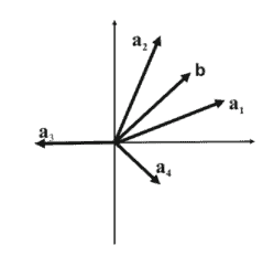
$\left(x_{1}, x_{2}, \ldots, x_{n}\right)$ is a feasible solution. Then, in terms of the columns of $\mathbf{A}$,
this solution satisfies:
$x_{1} \mathbf{a}{1}+x{2} \mathbf{a}{2}+\cdots+x{n} \mathbf{a}{n}=\mathbf{b} .$ Assume that exactly $p$ of the variables $x{i}$ are greater than zero, and for convenience,
that they are the first $p$ variables. Thus
$x_{1} \mathbf{a}{1}+x{2} \mathbf{a}{2}+\cdots+x{p} \mathbf{a}{p}=\mathbf{b}$ There are now two cases, corresponding as to whether the set $\mathbf{a}{1}, \mathbf{a}{2}, \ldots, \mathbf{a}{p}$ is
linearly independent or linearly dependent.
CASE 1: Assume $\mathbf{a}{1}, \mathbf{a}{2}, \ldots, \mathbf{a}{p}$ are linearly independent. Then clearly, $p \leqslant m$. If $p=m$, the solution is basic and the proof is complete. If $p{1}, \mathbf{a}{2}, \ldots, \mathbf{a}{p}$ are linearly dependent. Then there is a
nontrivial linear combination of these vectors that is zero. Thus there are constants $y_{1}, y_{2}, \ldots, y_{p}$, at least one of which can be assumed to be positive, such that
$y_{1}, y_{2}, \ldots, y_{p}$, at least one of which can be assumed to be positive, such that
$$
y_{1} \mathbf{a}{1}+y{2} \mathbf{a}{2}+\cdots+y{p} \mathbf{a}{p}=\mathbf{0} . $$ $y{1} \mathbf{a}{1}+y{2} \mathbf{a}{2}+\cdots+y{p} \mathbf{a}{p}=\mathbf{0} .$ Multiplying this equation by a scalar $\varepsilon$ and subtracting it from (2.14), we obtain $\left(x{1}-\varepsilon y_{1}\right) \mathbf{a}{1}+\left(x{2}-\varepsilon y_{2}\right) \mathbf{a}{2}+\cdots+\left(x{p}-\varepsilon y_{p}\right) \mathbf{a}{p}=\mathbf{b}$ This equation holds for every $\varepsilon$, and for each $\varepsilon$ the components $x{j}-\varepsilon y_{j}$ correspond
to a solution of the linear equalities-although they may violate $x_{i}-\varepsilon y_{i} \geqslant 0$.
Denoting $\mathbf{y}=\left(y_{1}, y_{2}, \ldots, y_{p}, 0,0, \ldots, 0\right)$, we see that for any $\varepsilon$
$\mathbf{x}-\varepsilon \mathbf{y}$
(2.17)
is a solution to the equalities. For $\varepsilon=0$, this reduces to the original feasible solution.
As $\varepsilon$ is increased from zero, the various components increase, decrease, or remain
As $\varepsilon$ is increased from zero, the various components increase, decrease, or remain
Since we assume at least one $y_{i}$ is positive, at least one component will decrease as $\varepsilon$
is increased. We increase $\varepsilon$ to the first point where one or more components become
zero. Specifically, we set
$\varepsilon=\min \left{x_{i} / y_{i}: y_{i}>0\right}$
$\varepsilon=\min \left{x_{i} / y_{i}: y_{i}>0\right}$
For this value of $\varepsilon$ the solution given by $(2.17)$ is feasible and has at most $p-1$
positive variables. Repeating this process if necessary, we can eliminate positive
variables until we have a feasible solution with corresponding columns that are
linearly independent. At that point Case 1 applies.
Proof of (ii) Let $\mathbf{x}=\left(x_{1}, x_{2}, \ldots, x_{n}\right)$ be an optimal feasible solution and, as in the
proof of (i) above, suppose there are exactly $p$ positive variables $x_{1}, x_{2}, \ldots, x_{p}$.
Again there are two cases; and Case 1, corresponding to linear independence, is
exactly the same as before.
Case 2 also goes exactly the same as before, but it must be shown that for any
$\varepsilon$ the solution $(2.17)$ is optimal. To show this, note that the value of the solution
在本节中,通过线性规划的基本定理,我们
确定基本可行解在求解线性问题中的首要重要性
程式。定理的证明方法在许多方面与
结果本身,因为它代表了单纯形发展的开始
方法。定理(由于 Carathéodory)本身表明它是必要的
在寻求线性的最优解时考虑基本可行解
程序,因为在这样的解决方案下总是可以达到最优值。
对应于标准形式的线性程序
最小化 $\mathbf{c}^{T} \mathbf{x}$
服从 $\mathbf{A x}=\mathbf{b}, \mathbf{x} \geqslant \mathbf{0}$
达到最小值的约束
(2.13)
达到最小值的约束的可行解
受这些约束的目标函数被称为最优可行
解决方案。如果这个解是基本的,则它是一个最优的基本可行解。
线性规划的基本定理给定标准线性规划
形式 (2.13) 其中 A 是一个秩为 $m$ 的 $m \times n$ 矩阵,
i) 若有可行解,则存在基本可行解; ii) 如果存在最优可行解,则存在最优基本可行解。
ii) 如果存在最优可行解,则存在最优基本可行解。
$\left(x_{1}, x_{2}, \ldots, x_{n}\right)$ 是一个可行的解决方案。那么,就 $\mathbf{A}$ 的列而言,
该解决方案满足:
$x_{1} \mathbf{a}{1}+x{2} \mathbf{a}{2}+\cdots+x{n} \mathbf{a}{n}=\mathbf{b } .$ 假设变量 $x{i}$ 中恰好有 $p$ 大于零,并且为方便起见,
它们是第一个 $p$ 变量。因此
$x_{1} \mathbf{a}{1}+x{2} \mathbf{a}{2}+\cdots+x{p} \mathbf{a}{p}=\mathbf{b }$ 现在有两种情况,分别对应集合 $\mathbf{a}{1}, \mathbf{a}{2}, \ldots, \mathbf{a}{p}$ 是否为
线性无关或线性相关。
情况 1:假设 $\mathbf{a}{1}、\mathbf{a}{2}、\ldots、\mathbf{a}{p}$ 是线性独立的。那么很明显,$p \leqslant m$。 如果$p=m$,则解是基本的,证明是完整的。如果 $p{1}、\mathbf{a}{2}、\ldots、\mathbf{a}{p}$ 是线性相关的。然后有一个
这些向量的非平凡线性组合为零。因此有常数$y_{1}, y_{2}, \ldots, y_{p}$,其中至少一个可以被假定为正数,使得
$y_{1}, y_{2}, \ldots, y_{p}$,其中至少一个可以假设为正数,使得
$$
y_{1} \mathbf{a}{1}+y{2} \mathbf{a}{2}+\cdots+y{p} \mathbf{a}{p}=\mathbf{0} . $$ $y{1} \mathbf{a}{1}+y{2} \mathbf{a}{2}+\cdots+y{p} \mathbf{a}{p}=\mathbf{0 } .$ 将这个方程乘以一个标量 $\varepsilon$ 并从 (2.14) 中减去它,我们得到 $\left(x{1}-\varepsilon y_{1}\right) \mathbf{a}{1}+\left(x{2}-\varepsilon y_{2}\right) \mathbf{a} {2}+\cdots+\left(x{p}-\varepsilon y_{p}\right) \mathbf{a}{p}=\mathbf{b}$ 这个等式对每一个 $\varepsilon$ 都成立,对于每一个 $\varepsilon$,分量 $x{j}-\varepsilon y_{j}$ 对应
线性等式的解——尽管它们可能违反$x_{i}-\varepsilon y_{i} \geqslant 0$。
表示 $\mathbf{y}=\left(y_{1}, y_{2}, \ldots, y_{p}, 0,0, \ldots, 0\right)$,我们看到对于任何 $\varepsilon $
$\mathbf{x}-\varepsilon \mathbf{y}$
(2.17)
是对等式的解决方案。对于$\varepsilon=0$,这简化为原始可行解。
随着 $\varepsilon$ 从零增加,各种成分增加、减少或保持
随着 $\varepsilon$ 从零增加,各种成分增加、减少或保持
因为我们假设至少有一个 $y_{i}$ 是正的,所以至少有一个分量会随着 $\varepsilon$ 而减少
增加。我们将 $\varepsilon$ 增加到一个或多个组件变为的第一个点
零。具体来说,我们设置
$\varepsilon=\min \left{x_{i} / y_{i}: y_{i}>0\right}$
$\varepsilon=\min \left{x_{i} / y_{i}: y_{i}>0\right}$
对于这个 $\varepsilon$ 的值,由 $(2.17)$ 给出的解是可行的并且最多有 $p-1$
正变量。如有必要重复此过程,我们可以消除阳性
变量,直到我们有一个可行的解决方案,对应的列是
线性独立。此时适用案例 1。
(ii) 的证明 令 $\mathbf{x}=\left(x_{1}, x_{2}, \ldots, x_{n}\right)$ 是最优可行解,如
上面 (i) 的证明,假设正好有 $p$ 个正变量 $x_{1}, x_{2}, \ldots, x_{p}$。
还有两种情况;情况 1,对应于线性独立,是
精确的
运筹学代考

什么是运筹学代写
运筹学(OR)是一种解决问题和决策的分析方法,在组织管理中很有用。在运筹学中,问题被分解为基本组成部分,然后通过数学分析按定义的步骤解决。
运筹学的过程大致可以分为以下几个步骤:
- 确定需要解决的问题。
- 围绕问题构建一个类似于现实世界和变量的模型。
- 使用模型得出问题的解决方案。
- 在模型上测试每个解决方案并分析其成功。
- 实施解决实际问题的方法。
与运筹学交叉的学科包括统计分析、管理科学、博弈论、优化理论、人工智能和复杂网络分析。所有这些学科的目标都是解决某一个现实中出现的复杂问题或者用数学的方法为决策提供指导。 运筹学的概念是在二战期间由参与战争的数学家们提出的。二战后,他们意识到在运筹学中使用的技术也可以被应用于解决商业、政府和社会中的问题。
运筹学代写的三个特点
所有运筹学解决实际问题的过程中都具有三个主要特征:
- 优化——运筹学的目的是在给定的条件下达到某一机器或者模型的最佳性能。优化还涉及比较不同选项和缩小潜在最佳选项的范围。
- 模拟—— 这涉及构建模型,以便在应用解决方案刀具体的复杂大规模问题之前之前尝试和测试简单模型的解决方案。
- 概率和统计——这包括使用数学算法和数据挖掘来发现有用的信息和潜在的风险,做出有效的预测并测试可能的解决方法。
运筹学领域提供了比普通软件和数据分析工具更强大的决策方法。此外,运筹学可以根据特定的业务流程或用例进行定制,以确定哪些技术最适合解决问题。
运筹学可以应用于各种活动,比如:计划和时间管理(Planning and Time Management),城乡规划(Urban and Rural Planning),企业资源计划(ERP)与供应链管理(Supply Chain Management)等等。 如有代写代考需求,欢迎同学们联系Assignmentexpert™,我们期待为你服务!