如果你也在 怎样代写图像处理Image Processing这个学科遇到相关的难题,请随时右上角联系我们的24/7代写客服。图像处理mage Processing的许多技术,或通常称为数字图片处理,是在20世纪60年代,在贝尔实验室、喷气推进实验室、麻省理工学院、马里兰大学和其他一些研究机构开发的,应用于卫星图像、有线照片标准转换、医学成像、可视电话、字符识别和照片增强。
图像处理作业Image Processing是使用数字计算机通过算法处理数字图像。 作为数字信号处理的一个子类别或领域,数字图像处理比模拟图像处理有许多优势。它允许更广泛的算法应用于输入数据,并能避免处理过程中的噪音和失真堆积等问题。由于图像是在两个维度(也许更多)上定义的,所以数字图像处理可以以多维系统的形式进行建模。数字图像处理的产生和发展主要受三个因素的影响:第一,计算机的发展;第二,数学的发展(特别是离散数学理论的创立和完善);第三,环境、农业、军事、工业和医学等方面的广泛应用需求增加。
my-assignmentexpert™ 图像处理Image Processing作业代写,免费提交作业要求, 满意后付款,成绩80\%以下全额退款,安全省心无顾虑。专业硕 博写手团队,所有订单可靠准时,保证 100% 原创。my-assignmentexpert™, 最高质量的图像处理Image Processing作业代写,服务覆盖北美、欧洲、澳洲等 国家。 在代写价格方面,考虑到同学们的经济条件,在保障代写质量的前提下,我们为客户提供最合理的价格。 由于统计Statistics作业种类很多,同时其中的大部分作业在字数上都没有具体要求,因此图像处理Image Processing作业代写的价格不固定。通常在经济学专家查看完作业要求之后会给出报价。作业难度和截止日期对价格也有很大的影响。
想知道您作业确定的价格吗? 免费下单以相关学科的专家能了解具体的要求之后在1-3个小时就提出价格。专家的 报价比上列的价格能便宜好几倍。
my-assignmentexpert™ 为您的留学生涯保驾护航 在数学mathematics作业代写方面已经树立了自己的口碑, 保证靠谱, 高质且原创的图像处理Image Processing作业代写代写服务。我们的专家在数学mathematics代写方面经验极为丰富,各种图像处理Image Processing相关的作业也就用不着 说。
我们提供的图像处理Image Processing及其相关学科的代写,服务范围广, 其中包括但不限于:

数学代写|图像处理作业代写Image Processing代考|Mean Square Error (MSE)
The investigation of the Mean Square Error (MSE) in classic periodogram analysis has a very long history. A single value of a periodogram has a large variance and MSE. The smoothing of a periodogram in the vicinity of a given frequency has been considered for the reduction of MSE. In addition, spectral windows for smoothing periodograms have been introduced by many authors, including Bartlett, Daniel, Parzen, Tukey, Hamming, Grenander, and Rosenblatt. However, the spectral windows designed by these authors have been used for both theoretical and practical purposes.
Our purpose is to determine the window with the smallest MSE for the smoothed periodogram $I(\lambda)$ over observed values $X(1), \ldots, X(N)$ of a stationary time series $X(t)$, with $t=\ldots 0,1,2, \ldots$, where $E(X(t))=$ constant $=0 \quad$ and $\quad \operatorname{Cov}(X(t+\tau), X(t))=C(\tau)$. The spectral representation of this time series is
$$
X(t)=\int_{-\pi}^{\pi} e^{i \lambda t} a(\lambda) d \lambda
$$
where $a(\lambda)$ is a random amplitude at frequency $\lambda$, such that $\operatorname{Cov}\left(a\left(\lambda_{1}\right), a\left(\lambda_{2}\right)\right)=0$ when $\lambda_{1} \neq \lambda_{2}$. The spectral density, $f(\lambda)$, is also known as the spectral energy at frequency $\lambda$ and is defined as
$$
f(\lambda)=E|a(\lambda)|^{2},-\pi<\lambda<\pi
$$
数学代写|图像处理作业代写Image Processing代考|The plots of functions O
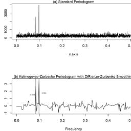
The coefficient closest to the optimal value appears to be the Kolmogorov estimation. The Kolmogorov estimation is a completely different type of estimation. The total number of observations, $N$, is divided into $T$ intersected segments, each length $M$, and a tapered $\mathrm{FT}$ is calculated at each segment. Tapering is performed by polynomial coefficients $a_{s}^{k, m}$, which may be interpreted as the distribution obtained by the convolution of $k$ uniform discrete distributions on the interval $[-(m-1) / 2,(m-1) / 2]$ such that $M=k(m-1)+1$. The squared, tapered FT is then averaged over $T$ consecutive segments. The asymptotic formula for the MSE of the Kolmogorov estimate is provided by Equation (1) with coefficient $k(\alpha)$. The Kolmogorov estimate has a low MSE and very high frequency resolution, as will be shown in more detail below (see Equations 2.1.2 and 2.1.3 as well as Equations 4.1.1 through 4.1.4). It can be generated through an iteration process, which makes it very computationally convenient.
数学代写|图像处理作业代写IMAGE PROCESSING代考|Application of KZ Filters on a Simulated Time Series
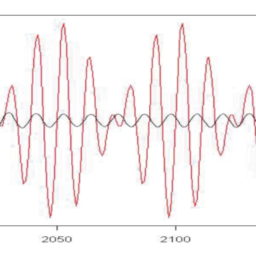
To demonstrate this approach, Zurbenko and Sowizral (1999) simulated a linear regression model $Y(t)=.9 X(t)+\varepsilon(t)$ by utilizing the following equations:
$$
\begin{aligned}
&X_{T}(t)=\operatorname{Cos}(2 \pi t / 1000) \
&Y_{T}(t)=.9 \operatorname{Cos}(2 \pi t / 1000)+.5 \operatorname{Sin}(2 \pi t / 1000)
\end{aligned}
$$
with $\sin (2 \pi t / 1000)$ and $\cos (2 \pi t / 1000)$ uncorrelated and $t=$ $0,1, \ldots, 2999$. To test the effect of noise on the regression, normal noise was added with mean 0 and variance 9 , such that
$$
\begin{aligned}
&X_{T}(t)=\operatorname{Cos}(2 \pi t / 1000)+N(0,9) \
&Y_{T}(t)=.9 \operatorname{Cos}(2 \pi t / 1000)+.5 \operatorname{Sin}(2 \pi t / 1000)+N(0,9)
\end{aligned}
$$
where $N(0,9)$ is normal noise and $t=0,1, \ldots, 2999$.
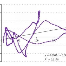
Figure 2.2.1 presents the combined scatterplots of the data with and without noise. While the slope of the regression line for data without noise has a near perfect slope $(m=0.900)$, the slope of the regression line for data with noise is close to $0(m=0.033)$.
图像处理代写
数学代写|图像处理作业代写IMAGE PROCESSING代考|MEAN SQUARE ERROR米小号和
均方误差的调查米小号和在经典的周期图分析中有很长的历史。周期图的单个值具有较大的方差和 MSE。已考虑在给定频率附近平滑周期图以降低 MSE。此外,许多作者已经引入了用于平滑周期图的光谱窗口,包括 Bartlett、Daniel、Parzen、Tukey、Hamming、Grenander 和 Rosenblatt。然而,这些作者设计的光谱窗口已被用于理论和实际目的。
我们的目的是为平滑周期图确定具有最小 MSE 的窗口一世(λ)超过观察值X(1),…,X(ñ)平稳时间序列的X(吨), 和吨=…0,1,2,…, 在哪里和(X(吨))=持续的=0和这(X(吨+τ),X(吨))=C(τ). 这个时间序列的光谱表示是
X(吨)=∫−圆周率圆周率和一世λ吨一种(λ)dλ
在哪里一种(λ)是频率上的随机幅度λ, 这样这(一种(λ1),一种(λ2))=0什么时候λ1≠λ2. 光谱密度,F(λ), 也称为频率处的光谱能量λ并定义为
F(λ)=和|一种(λ)|2,−圆周率<λ<圆周率
数学代写|图像处理作业代写IMAGE PROCESSING代考|THE PLOTS OF FUNCTIONS O
最接近最优值的系数似乎是 Kolmogorov 估计。Kolmogorov 估计是一种完全不同的估计类型。观察总数,ñ, 分为吨相交的段,每个长度米, 和一个锥形F吨在每个段计算。锥化由多项式系数执行一种s到,米,这可以解释为通过卷积得到的分布到区间上的均匀离散分布[−(米−1)/2,(米−1)/2]这样米=到(米−1)+1. 然后对平方的锥形 FT 进行平均吨连续的段。Kolmogorov 估计的 MSE 的渐近公式由方程提供1有系数到(一种). Kolmogorov 估计具有低 MSE 和非常高的频率分辨率,如下面将更详细地展示s和和和q你一种吨一世这ns2.1.2一种nd2.1.3一种s在和一世一世一种s和q你一种吨一世这ns4.1.1吨Hr这你GH4.1.4. 它可以通过迭代过程生成,这使得它在计算上非常方便。
数学代写|图像处理作业代写IMAGE PROCESSING代考|APPLICATION OF KZ FILTERS ON A SIMULATED TIME SERIES
为了演示这种方法,Zurbenko 和 Sowizral1999模拟线性回归模型是(吨)=.9X(吨)+e(吨)通过利用以下等式:
X吨(吨)=某物(2圆周率吨/1000) 是吨(吨)=.9某物(2圆周率吨/1000)+.5没有(2圆周率吨/1000)
和没有(2圆周率吨/1000)和某物(2圆周率吨/1000)不相关和吨= 0,1,…,2999. 为了测试噪声对回归的影响,添加了均值为 0 和方差为 9 的正态噪声,使得
X吨(吨)=某物(2圆周率吨/1000)+ñ(0,9) 是吨(吨)=.9某物(2圆周率吨/1000)+.5没有(2圆周率吨/1000)+ñ(0,9)
在哪里ñ(0,9)是正常的噪音和吨=0,1,…,2999.
图 2.2.1 显示了有噪声和无噪声数据的组合散点图。虽然没有噪声的数据的回归线的斜率具有近乎完美的斜率(米=0.900),有噪声数据的回归线的斜率接近0(米=0.033).

matlab代写请认准UprivateTA™. UprivateTA™为您的留学生涯保驾护航。