如果你也在 怎样代写图像处理Image Processing这个学科遇到相关的难题,请随时右上角联系我们的24/7代写客服。图像处理mage Processing的许多技术,或通常称为数字图片处理,是在20世纪60年代,在贝尔实验室、喷气推进实验室、麻省理工学院、马里兰大学和其他一些研究机构开发的,应用于卫星图像、有线照片标准转换、医学成像、可视电话、字符识别和照片增强。
图像处理作业Image Processing是使用数字计算机通过算法处理数字图像。 作为数字信号处理的一个子类别或领域,数字图像处理比模拟图像处理有许多优势。它允许更广泛的算法应用于输入数据,并能避免处理过程中的噪音和失真堆积等问题。由于图像是在两个维度(也许更多)上定义的,所以数字图像处理可以以多维系统的形式进行建模。数字图像处理的产生和发展主要受三个因素的影响:第一,计算机的发展;第二,数学的发展(特别是离散数学理论的创立和完善);第三,环境、农业、军事、工业和医学等方面的广泛应用需求增加。
my-assignmentexpert™ 图像处理Image Processing作业代写,免费提交作业要求, 满意后付款,成绩80\%以下全额退款,安全省心无顾虑。专业硕 博写手团队,所有订单可靠准时,保证 100% 原创。my-assignmentexpert™, 最高质量的图像处理Image Processing作业代写,服务覆盖北美、欧洲、澳洲等 国家。 在代写价格方面,考虑到同学们的经济条件,在保障代写质量的前提下,我们为客户提供最合理的价格。 由于统计Statistics作业种类很多,同时其中的大部分作业在字数上都没有具体要求,因此图像处理Image Processing作业代写的价格不固定。通常在经济学专家查看完作业要求之后会给出报价。作业难度和截止日期对价格也有很大的影响。
想知道您作业确定的价格吗? 免费下单以相关学科的专家能了解具体的要求之后在1-3个小时就提出价格。专家的 报价比上列的价格能便宜好几倍。
my-assignmentexpert™ 为您的留学生涯保驾护航 在数学mathematics作业代写方面已经树立了自己的口碑, 保证靠谱, 高质且原创的图像处理Image Processing作业代写代写服务。我们的专家在数学mathematics代写方面经验极为丰富,各种图像处理Image Processing相关的作业也就用不着 说。
我们提供的图像处理Image Processing及其相关学科的代写,服务范围广, 其中包括但不限于:
数学代写|图像处理作业代写Image Processing代考|The KZ filter: Identifying and separating scales of influence in data
The KZ filter is a low-pass filter which is designed based on spectral characteristics. It is constructed as an iterated moving average filter. The user sets the number of times, $k$, to iterate the moving average, and the number of points, $m$, to include in each iteration. These parameters should, in turn, be determined based on the spectral scales that the user wishes to separate. The $\mathrm{KZ}(m, k)$ filter applied to the discrete stochastic process $X(t)$, $\mathrm{t}=0, \pm 1, \pm 2, \ldots$, is then defined recursively as
$$
\begin{aligned}
\mathrm{KZ}(m, 1)[X(t)]=& \frac{1}{m} \sum_{s=-(m-1) / 2}^{(m-1) / 2} X(t+s) \
\mathrm{KZ}(m, k)[X(t)]=& \frac{1}{m} \sum_{s=-(m-1) / 2}^{(m-1) / 2} \mathrm{KZ}(m, k-1)[X(t\
&+s)], k \geq 2 .
\end{aligned}
$$
When some of the data within the m-point interval is missing, the missing observations may simply be ignored, and the average then taken over the points available within the interval. The impulse response function of the filter has support over $k(m-1)+1$ points, has $k$ – 2 continuous derivatives which approach zero at the edges of the support, and approaches the Gaussian distribution as $k$ is made large. As such, it tapers sharply outside $\pm \frac{1}{2} m \sqrt{k}$, yielding a high-resolution cut-off in the frequency domain. $.^{21,22}$ The filter’s squared transfer function is
$$
\left|\phi_{m, k}(\omega)\right|^{2}=\left[\frac{\sin (\pi m \omega)}{m \sin (\pi \omega)}\right]^{2 k}
$$
Here, $\omega$ is the frequency, or the number of cycles per unit of time or space. As $k$ is increased, the spectral leakage is increasingly damped, so that $k$ controls the sharpness of frequency resolution. The parameter $m$ is set according to the desired cut-off frequency, which we denote as $\omega^{}$. To attain a cut-off frequency close to $\omega^{}$, set $m$ such that $\left|\phi_{m, k}\left(\omega^{*}\right)\right|^{2} \approx .5 .^{15}$
数学代写|图像处理作业代写Image Processing代考|Signal reconstruction in time and space: removing noise and detecting break points
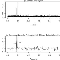
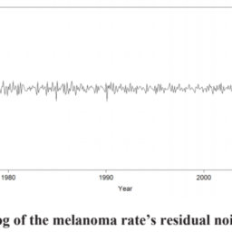
Given a signal organized in time and/or space, a break point is a discontinuity jump in the signal’s long-term trend component. In real world data, breakpoints are often obscured by noise and smooth changes occurring in the unfiltered data. Break points are frequently observed in natural data, and may correspond to a sudden change in measurements due to measurement tool replacement, a policy change impacting how measurements are defined, or a real, physical change in the system being measured, such as a disease outbreak or a market crash. Often, the break’s position in time and/or space is unknown a priori, and the confluence of noisy short-term components and seasonal and longer term fluctuations make the break invisible to the eye in raw data.The $\mathrm{KZ}$ adaptive (KZA) algorithm is designed to reveal breakpoints in time and space, and is able to determine their precise size and location. ${ }^{1,33}$ The algorithm works by monitoring abrupt changes in signal smoothness through the application of a KZ filter. If such a change is detected, the algorithm then adapts the size of the moving average window to treat the data before and after the detected breakpoint separately. Recall that the KZ filter uses a centered moving average. Informally, the KZA algorithm separates the moving average window into its head and tail, respectively defined as the points in the moving average window to the right and left of the center point. As the center of the moving average window approaches the breakpoint from the left, the size of the head of the moving average window shrinks, so that the moving average window is composed of points only to the left of the breakpoint. Then, as the center of the moving average window passes the breakpoint, the head stretches out again to its full size, and the tail shrinks, so that the moving average window contains points only to the right of the breakpoint.
数学代写|图像处理作业代写IMAGE PROCESSING代考|Application: Spatio-temporal analysis of global climate fluctuations
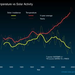
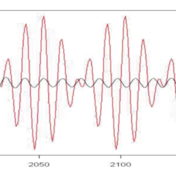
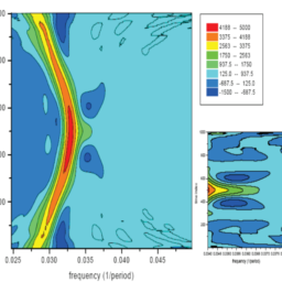
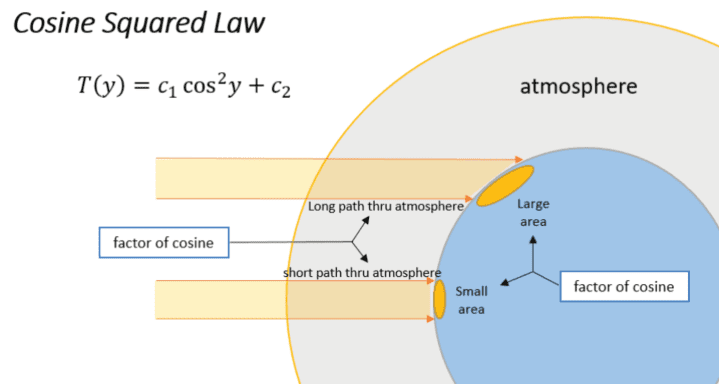
The application of a multidimensional $\mathrm{KZ}$ filter yields a function of the same dimension, which contains only the low frequency scale components of the signal and where the frequency cutoff is determined by the filter’s parameters. Zurbenko and Cyr used the multidimensional $\mathrm{KZ}$ filter to separate the different scales that compose global climate fluctuations. ${ }^{24} \mathrm{In}$ this paper, the DZ algorithm facilitated high resolution spectral analysis of global temperature data $T(x, y, t)$, which uncovered two frequencies lower than the temperature data’s seasonal component: an 11-13 years period and a $2-5$ years period. The 11-13 years period is the result of an 11-13 year periodicity in solar activity, and the $2-5$ years period corresponds to the well-known El Niño oscillations. The periodic components were separated using KZ filters, as described in Section 6.1. The 11-13 year period had global spatial scale and was correlated in time with sunspot data, which Zurbenko and Potrzeba-Macrina $(2019)^{29}$ proved are proportional to solar irradiation levels on earth; however, in the last few decades, the global temperature component began to increase out of step with sunspot data. It was also shown that this global temperature component is remarkably wellordered with latitude $y$ and is linearly approximated with accuracy exceeding $99 \%$ by the relation $T_{g}(y)=a_{1} \cos ^{2} y+a_{0}$, where $T_{g}$ is taken to be the global temperature component. If the temperature is measured in Fahrenheit, then Zurbenko and Cyr estimate $a_{0}=12.94$ and $a_{1}=63.35 .^{24}$ This latitudinal description of the global temperature component is called the cosine squared law, which describes how global temperature over latitudes is affected simultaneously by the angle between the latitude $y$ and the sun, and the length of the path through the atmosphere at latitude $y$, with each of these effects causing a factor of $\cos y$ in the linear relation above. This is depicted below in Figure 6.3.1.
图像处理代写
数学代写|图像处理作业代写IMAGE PROCESSING代考|THE KZ FILTER: IDENTIFYING AND SEPARATING SCALES OF INFLUENCE IN DATA
KZ滤波器是一种基于光谱特性设计的低通滤波器。它被构造为迭代移动平均滤波器。用户设置次数,到, 迭代移动平均线和点数,米, 包含在每次迭代中。反过来,这些参数应该根据用户希望分离的光谱尺度来确定。这到从(米,到)应用于离散随机过程的滤波器X(吨),吨=0,±1,±2,…, 然后递归定义为
到从(米,1)[X(吨)]=1米∑s=−(米−1)/2(米−1)/2X(吨+s) 到从(米,到)[X(吨)]=1米∑s=−(米−1)/2(米−1)/2到从(米,到−1)[X(吨 +s)],到≥2.
当 m 点区间内的某些数据缺失时,可以简单地忽略缺失的观测值,然后取平均值取区间内可用的点。滤波器的脉冲响应函数支持超过到(米−1)+1点,有到– 2 个连续导数,在支持的边缘接近零,并接近高斯分布到变大了。因此,它在外部急剧变细±12米到,在频域中产生高分辨率截止。.21,22滤波器的平方传递函数为
|φ米,到(ω)|2=[没有(圆周率米ω)米没有(圆周率ω)]2到
这里,ω是频率,或每单位时间或空间的周期数。作为到增加,频谱泄漏越来越衰减,所以到控制频率分辨率的锐度。参数米根据所需的截止频率设置,我们将其表示为 $\omega^{ }.吨这一种吨吨一种一世n一种C你吨−这FFFr和q你和nC是C一世这s和吨这\欧米茄^{ },s和吨米s你CH吨H一种吨\左|\phi_{m, k}\左\omega^{*}\右\omega^{*}\右\right|^{2} \约 .5 .^{15}$
数学代写|图像处理作业代写IMAGE PROCESSING代考|SIGNAL RECONSTRUCTION IN TIME AND SPACE: REMOVING NOISE AND DETECTING BREAK POINTS
给定按时间和/或空间组织的信号,断点是信号长期趋势分量中的不连续跳跃。在现实世界的数据中,断点经常被未经过滤的数据中发生的噪声和平滑变化所掩盖。在自然数据中经常观察到断点,并且可能对应于由于测量工具更换而导致的测量突然变化、影响测量定义方式的政策变化或被测量系统中的真实物理变化,例如疾病爆发或市场崩盘。通常,中断在时间和/或空间中的位置是先验未知的,并且嘈杂的短期成分以及季节性和长期波动的汇合使得原始数据中的中断对眼睛是不可见的。到从自适应到从一种算法旨在揭示时间和空间上的断点,并能够确定它们的精确大小和位置。1,33该算法通过应用 KZ 滤波器来监控信号平滑度的突然变化。如果检测到这样的变化,则算法会调整移动平均窗口的大小,以分别处理检测到的断点之前和之后的数据。回想一下,KZ 滤波器使用居中移动平均线。通俗地说,KZA 算法将移动平均窗口分为头部和尾部,分别定义为移动平均窗口中位于中心点左右的点。随着移动平均窗口的中心从左侧接近断点,移动平均窗口的头部尺寸缩小,使得移动平均窗口仅由断点左侧的点组成。然后,随着移动平均窗口的中心通过断点,
数学代写|图像处理作业代写IMAGE PROCESSING代考|APPLICATION: SPATIO-TEMPORAL ANALYSIS OF GLOBAL CLIMATE FLUCTUATIONS
多维应用到从filter 产生一个相同维度的函数,它只包含信号的低频尺度分量,并且频率截止由滤波器的参数确定。Zurbenko 和 Cyr 使用多维到从过滤以分离构成全球气候波动的不同尺度。24一世n本文,DZ 算法促进了全球温度数据的高分辨率光谱分析吨(X,是,吨),它揭示了两个频率低于温度数据的季节性成分:11-13 年的周期和2−5年期间。11-13 年周期是太阳活动 11-13 年周期的结果,而2−5年周期对应于著名的厄尔尼诺振荡。如第 6.1 节所述,使用 KZ 滤波器分离周期性分量。11-13 年期间具有全球空间尺度,并与太阳黑子数据在时间上相关,其中 Zurbenko 和 Potrzeba-Macrina(2019)29证明与地球上的太阳辐射水平成正比;然而,在过去的几十年里,全球温度分量的增加开始与太阳黑子数据不同步。还表明,这个全球温度分量与纬度非常有序是并且是线性近似的,精度超过99%由关系吨G(是)=一种1某物2是+一种0, 在哪里吨G被视为全球温度分量。如果温度以华氏度为单位,则 Zurbenko 和 Cyr 估计一种0=12.94和一种1=63.35.24这种对全球温度分量的纬度描述称为余弦平方定律,它描述了纬度上的全球温度如何同时受到纬度之间的角度的影响是和太阳,以及在纬度上穿过大气层的路径长度是,这些影响中的每一个都会导致某物是在上面的线性关系中。这在下面的图 6.3.1 中进行了描述。

matlab代写请认准UprivateTA™. UprivateTA™为您的留学生涯保驾护航。