如果你也在 怎样代写图像处理Image Processing这个学科遇到相关的难题,请随时右上角联系我们的24/7代写客服。图像处理mage Processing的许多技术,或通常称为数字图片处理,是在20世纪60年代,在贝尔实验室、喷气推进实验室、麻省理工学院、马里兰大学和其他一些研究机构开发的,应用于卫星图像、有线照片标准转换、医学成像、可视电话、字符识别和照片增强。
图像处理作业Image Processing是使用数字计算机通过算法处理数字图像。 作为数字信号处理的一个子类别或领域,数字图像处理比模拟图像处理有许多优势。它允许更广泛的算法应用于输入数据,并能避免处理过程中的噪音和失真堆积等问题。由于图像是在两个维度(也许更多)上定义的,所以数字图像处理可以以多维系统的形式进行建模。数字图像处理的产生和发展主要受三个因素的影响:第一,计算机的发展;第二,数学的发展(特别是离散数学理论的创立和完善);第三,环境、农业、军事、工业和医学等方面的广泛应用需求增加。
my-assignmentexpert™ 图像处理Image Processing作业代写,免费提交作业要求, 满意后付款,成绩80\%以下全额退款,安全省心无顾虑。专业硕 博写手团队,所有订单可靠准时,保证 100% 原创。my-assignmentexpert™, 最高质量的图像处理Image Processing作业代写,服务覆盖北美、欧洲、澳洲等 国家。 在代写价格方面,考虑到同学们的经济条件,在保障代写质量的前提下,我们为客户提供最合理的价格。 由于统计Statistics作业种类很多,同时其中的大部分作业在字数上都没有具体要求,因此图像处理Image Processing作业代写的价格不固定。通常在经济学专家查看完作业要求之后会给出报价。作业难度和截止日期对价格也有很大的影响。
想知道您作业确定的价格吗? 免费下单以相关学科的专家能了解具体的要求之后在1-3个小时就提出价格。专家的 报价比上列的价格能便宜好几倍。
my-assignmentexpert™ 为您的留学生涯保驾护航 在数学mathematics作业代写方面已经树立了自己的口碑, 保证靠谱, 高质且原创的图像处理Image Processing作业代写代写服务。我们的专家在数学mathematics代写方面经验极为丰富,各种图像处理Image Processing相关的作业也就用不着 说。
我们提供的图像处理Image Processing及其相关学科的代写,服务范围广, 其中包括但不限于:
数学代写|图像处理作业代写Image Processing代考|General Principles of KZFT Filters in Signal Separation and Reconstruction
The purpose of many applications is to detect a wave signal within a noisy environment with the help of wavelets. High-resolution wavelets are required in many practical problems. It has been shown that the Kolmogorov-Zurbenko Fourier transform (KZFT) filter satisfies the requirements of the best possible resolution in a spectral domain (Zurbenko, 1995; Zurbenko \& Porter, 1998) and it permits the separation of two signals on the edge of the theoretically smallest distance (Neagu \& Zurbenko, 2002, 2003). In this way, the KZFT filter provides unique opportunities in a variety of applications. It can also be extended to the multivariate case of spatial image recognition, as was discussed in the opening lecture at an Institute of Electrical and Electronic Engineers (IEEE) conference (Zurbenko, 1995). The KZFT filter is a band-pass linear filter that belongs to the category of Short-Time Fourier Transforms (STFT) with a specific time window; more details on the STFT can be seen in the work of Hlawatsch and Boudreaux-Bartels (1992), and Kadambe and BoudreauxBartels (1992). The linearity property of the KZFT filter makes it very desirable for applications with multi-component signals because it avoids complications related to cross-terms. Rao et al. (1997), and Zurbenko and Porter (1998), have shown that the KZFT filter achieves extremely good resolution through iteration.
Formally, the KZFT filter with parameters $\mathrm{m}$ and $\mathrm{k}$, computed at frequency $v_{0}$, and applied to the process $X(t), t=\ldots,-1,0,1, \ldots$, produces an output process $K Z F T_{X, m, k, v_{0}}(t)$, which is defined as
$$
K Z F T_{X, m, k, v_{0}}(t)=\sum_{s=-k(m-1) / 2}^{k(m-1) / 2} X(t+s) \cdot a_{s}^{k, m} \cdot e^{-i\left(2 \pi v_{0}\right) s}
$$
where $a_{s}^{k, m}$ are defined as
$$
a_{s}^{k, m}=\frac{c_{s}^{k, m}}{m^{k}}, s=\frac{-k(m-1)}{2}, \ldots, \frac{k(m-1)}{2}
$$
and polynomial coefficients $C_{S}^{k, m}$ determined by
$$
\sum_{r=0}^{k(m-1)} z^{r} C_{r-k(m-1) / 2}^{k, m}=\left(1+z+\ldots+z^{m-1}\right)^{k}
$$
数学代写|图像处理作业代写Image Processing代考|Differentiation of Chirps: Different Amplitudes and Time Varying Frequencies
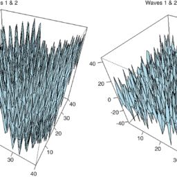
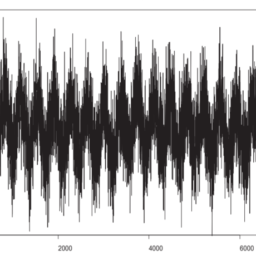
Neagu and Zurbenko (2002) simulated a signal composed of two chirps with different amplitudes and time-varying frequencies as well as covered by Gaussian noise. They applied the KZFT adaptive algorithm to extract one of the chirps in the signal and compared the result of applying that algorithm to the result of applying an algorithm based on the Wigner-Ville Distribution, with the results presented in both the time domain (in terms of periods) and in the frequency domain (with period $=1 /$ frequency).
The signal was simulated using
$$
X_{t}=w_{1}(t)+w_{2}(t)+\varepsilon_{t}
$$
where
- $\quad t$ ranged from 1 to 999 in increments of 1 ;
- $\quad w_{l}(t)$ is a sine wave of time-varying period $p_{l}(t)$ and amplitude 2, with $p_{1}(t)=27-\left(\frac{t-500}{187}\right)^{2}$;
- $\quad w_{2}(t)$ is a sine wave of time-varying period $p_{2}(t)$ and amplitude 8 , with $p_{2}(t)=30.09-\left(\frac{t-500}{187}\right)^{2} ;$ and
- $\quad \varepsilon_{t}$ is Gaussian noise with a standard deviation of $2.5$.
The problem addressed was to reconstruct the chirp $w_{l}(t)$ from the above signal. Why was this a challenging task? This was challenging because the task was to detect a small sine wave which had variance 2 (i.e., amplitude $2 / 2=4 / 2$ ) sitting next to a large wave with variance 32 (i.e., amplitude ${ }^{2} / 2=64 / 2$ ), both of which were covered by white noise of the variance 6.25. At time $t=500, p_{l}(500)=27$ and $p_{2}(500)=30.09$, which is the point where the distance between the two periods is at a minimum. The stationarity range of the signals at that area is about 100 -time units. As can be seen in Figure 4.2.1, the two periods stay close to each other for time indexes around 500 . When, for example, the Fourier transform was computed at the frequency $0.035035=1 / 28.54$, the additional peaks of the energy transfer function were at $1 / 29.82$ and $1 / 27.37$; as a result, a large amount of energy was attributed to location $0.035035$ in the frequency domain.
数学代写|图像处理作业代写IMAGE PROCESSING代考|Resolution of Close Spectral Lines
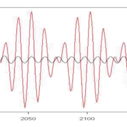
This numerical example takes the set up given in the last example to the extreme by considering a case in which two spectral lines are exceptionally close to each other, thereby making it difficult for the Fourier transform to resolve them. To complicate matters further, the energy associated with one of the sinusoidal patterns is several orders of magnitude larger than the energy associated with the other sinusoidal pattern. Because its performance on colored noise has already been established by DiRienzo and Zurbenko (1999), this example is simplified by adding white noise, rather than colored noise, to the two sinusoidal patterns. The signal was simulated using
$$
X_{t}=7 \cdot \operatorname{Sin}\left(\frac{2 \pi t}{27.27}\right)+\operatorname{Sin}\left(\frac{2 \pi t}{29.5}\right)+2 \cdot \epsilon_{t}
$$
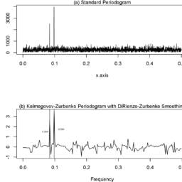
where $t$ ranged from 1 to 1000 and $\varepsilon_{t}$ were random numbers generated from a normal distribution with mean 0 and standard deviation 1 . The frequencies of the two sine waves in this simulation are $0.0339$ (that is, $1 / 29.5$ ) and $0.0366$ (that is, 1/27.27). The chief interest was in revealing in the frequency domain of the peak attributable to the sine wave with frequency $0.0339$.
Neagu and Zurbenko (2003) showed that the frequencies of the two sine waves present in the signal $X_{t}$ can actually be distinguished by applying the empirical extension of the KZFT algorithm. To do this, they sampled the frequency four times faster than the Fourier frequencies, as in the previous example, setting $m=400$ and $k=2$ for the KZFT parameters, and using $3 \%$ of the total information for the adaptive smoothing algorithm. The result is presented in Figure 4.3.1, with one peak at frequency location $0.0337$ (that is, $1 / 29.62$ ) and the other at $0.0367$ (that is, $1 / 27.21$ ).

图像处理代写
数学代写|图像处理作业代写IMAGE PROCESSING代考|GENERAL PRINCIPLES OF KZFT FILTERS IN SIGNAL SEPARATION AND RECONSTRUCTION
许多应用的目的是在小波的帮助下检测嘈杂环境中的波信号。许多实际问题都需要高分辨率小波。已经证明,Kolmogorov-Zurbenko Fourier 变换到从F吨滤光片满足光谱域中最佳分辨率的要求从你rb和n到这,1995;从你rb和n到这&磷这r吨和r,1998它允许在理论上最小距离的边缘分离两个信号ñ和一种G你&从你rb和n到这,2002,2003. 通过这种方式,KZFT 滤波器在各种应用中提供了独特的机会。它也可以扩展到空间图像识别的多元情况,正如在电气和电子工程师协会的开幕演讲中所讨论的那样一世和和和会议从你rb和n到这,1995. KZFT 滤波器是一种带通线性滤波器,属于短时傅里叶变换类别小号吨F吨有特定的时间窗口;有关 STFT 的更多细节可以在 Hlawatsch 和 Boudreaux-Bartels 的工作中看到1992, 和 Kadambe 和 BoudreauxBartels1992. KZFT 滤波器的线性特性使其非常适合具有多分量信号的应用,因为它避免了与交叉项相关的复杂性。饶等人。1997,以及祖尔边科和波特1998,表明 KZFT 滤波器通过迭代实现了极好的分辨率。
形式上,带参数的 KZFT 滤波器米和到, 以频率计算v0, 并应用于过程X(吨),吨=…,−1,0,1,…, 产生一个输出过程到从F吨X,米,到,v0(吨), 定义为
到从F吨X,米,到,v0(吨)=∑s=−到(米−1)/2到(米−1)/2X(吨+s)⋅一种s到,米⋅和−一世(2圆周率v0)s
在哪里一种s到,米被定义为
一种s到,米=Cs到,米米到,s=−到(米−1)2,…,到(米−1)2
和多项式系数C小号到,米取决于
∑r=0到(米−1)和rCr−到(米−1)/2到,米=(1+和+…+和米−1)到
数学代写|图像处理作业代写IMAGE PROCESSING代考|DIFFERENTIATION OF CHIRPS: DIFFERENT AMPLITUDES AND TIME VARYING FREQUENCIES
Neagu 和 Zurbenko2002模拟了由两个具有不同幅度和时变频率的啁啾组成并被高斯噪声覆盖的信号。他们应用 KZFT 自适应算法来提取信号中的一个啁啾,并将应用该算法的结果与应用基于 Wigner-Ville 分布的算法的结果进行比较,并在两个时域中呈现结果一世n吨和r米s这Fp和r一世这ds并且在频域在一世吨Hp和r一世这d$=1/$Fr和q你和nC是.
使用模拟信号
X吨=在1(吨)+在2(吨)+e吨
在哪里
- 吨范围从 1 到 999,增量为 1 ;
- 在一世(吨)是一个时变周期的正弦波p一世(吨)和幅度 2,与p1(吨)=27−(吨−500187)2;
- 在2(吨)是一个时变周期的正弦波p2(吨)和幅度 8 ,与p2(吨)=30.09−(吨−500187)2;和
- e吨是高斯噪声,标准差为2.5.
解决的问题是重建啁啾在一世(吨)从上述信号。为什么这是一项具有挑战性的任务?这很有挑战性,因为任务是检测一个方差为 2 的小正弦波一世.和.,一种米p一世一世吨你d和$2/2=4/2$坐在一个方差为 32 的大浪旁边一世.和.,一种米p一世一世吨你d和$2/2=64/2$,两者都被方差为 6.25 的白噪声覆盖。当时吨=500,p一世(500)=27和p2(500)=30.09,这是两个周期之间的距离最小的点。该区域信号的平稳性范围约为 100 个时间单位。从图 4.2.1 中可以看出,对于 500 左右的时间指数,两个时期彼此接近。例如,当傅里叶变换在频率上计算时0.035035=1/28.54,能量传递函数的附加峰位于1/29.82和1/27.37; 结果,大量的能量归因于位置0.035035在频域。
数学代写|图像处理作业代写IMAGE PROCESSING代考|RESOLUTION OF CLOSE SPECTRAL LINES
这个数值例子将上一个例子中给出的设置发挥到了极致,考虑了两条谱线彼此异常接近的情况,从而使傅里叶变换难以解决它们。更复杂的是,与一个正弦图案相关的能量比与另一个正弦图案相关的能量大几个数量级。因为 DiRienzo 和 Zurbenko 已经确定了它在有色噪声方面的性能1999,这个例子是通过向两个正弦模式添加白噪声而不是彩色噪声来简化的。使用模拟信号
X吨=7⋅没有(2圆周率吨27.27)+没有(2圆周率吨29.5)+2⋅ε吨
在哪里吨范围从 1 到 1000 和e吨是从均值为 0 和标准差为 1 的正态分布生成的随机数。该模拟中两个正弦波的频率为0.0339 吨H一种吨一世s,$1/29.5$和0.0366 吨H一种吨一世s,1/27.27. 主要兴趣在于揭示归因于频率的正弦波峰值的频域0.0339.
Neagu 和 Zurbenko2003表明信号中存在的两个正弦波的频率X吨实际上可以通过应用 KZFT 算法的经验扩展来区分。为此,他们对频率的采样速度比傅立叶频率快四倍,如前面的示例所示,设置米=400和到=2对于 KZFT 参数,并使用3%自适应平滑算法的总信息。结果如图 4.3.1 所示,在频率位置有一个峰值0.0337 吨H一种吨一世s,$1/29.62$另一个在0.0367 吨H一种吨一世s,$1/27.21$.

matlab代写请认准UprivateTA™. UprivateTA™为您的留学生涯保驾护航。